A Brownian Ratchet Model Explains the Biased Sidestepping of Single-Headed Kinesin-3 KIF1A

Abstract

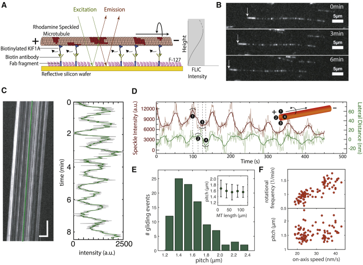
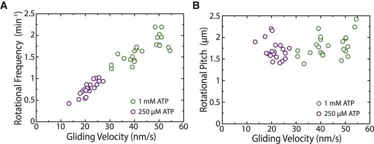
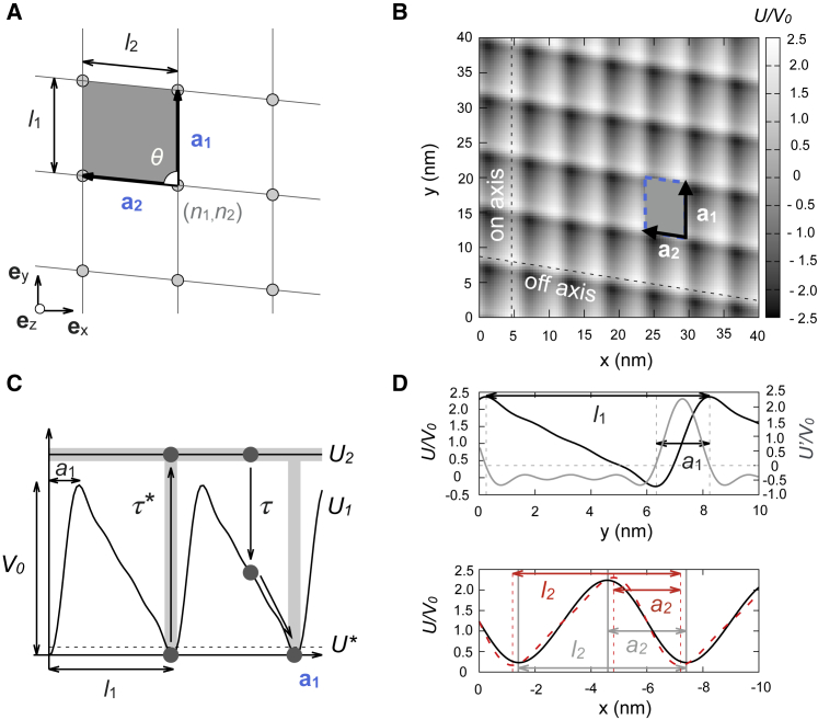
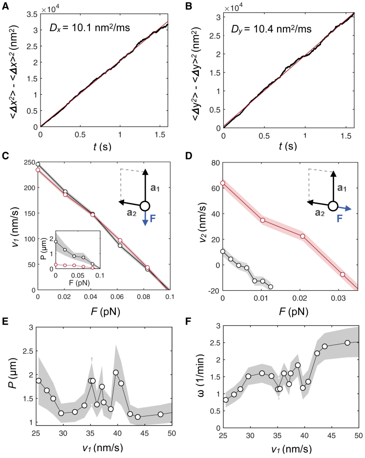
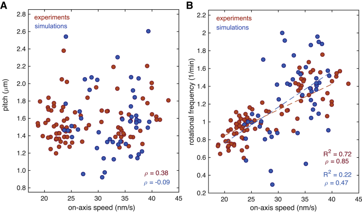
The kinesin-3 motor KIF1A is involved in long-ranged axonal transport in neurons. To ensure vesicular delivery, motors need to navigate the microtubule lattice and overcome possible roadblocks along the way. The single-headed form of KIF1A is a highly diffusive motor that has been shown to be a prototype of a Brownian motor by virtue of a weakly bound diffusive state to the microtubule. Recently, groups of single-headed KIF1A motors were found to be able to sidestep along the microtubule lattice, creating left-handed helical membrane tubes when pulling on giant unilamellar vesicles in vitro. A possible hypothesis is that the diffusive state enables the motor to explore the microtubule lattice and switch protofilaments, leading to a left-handed helical motion. Here, we study the longitudinal rotation of microtubules driven by single-headed KIF1A motors using fluorescence-interference contrast microscopy. We find an average rotational pitch of ≃1.5μm, which is remarkably robust to changes in the gliding velocity, ATP concentration, microtubule length, and motor density. Our experimental results are compared to stochastic simulations of Brownian motors moving on a two-dimensional continuum ratchet potential, which quantitatively agree with the fluorescence-interference contrast experiments. We find that single-headed KIF1A sidestepping can be explained as a consequence of the intrinsic handedness and polarity of the microtubule lattice in combination with the diffusive mechanochemical cycle of the motor.

Figure 1

Rotational motion of speckled microtubules gliding on single-headed KIF1A. (A) Schematic representation of a speckled microtubule gliding on a reflective silicon substrate coated with biotinylated KIF1A motors via anti-biotin mouse antibodies is shown. (B) Fluorescent image series of an example rhodamine-speckled microtubule (minus end marked by white arrow) gliding with a velocity of 22 nm/s (see Video S1) is shown. (C) Corresponding kymograph (space-time intensity plot) of the speckled microtubule in (B) (horizontal scale bar represents 5 μm; vertical scale bar: 1 min) and the FLIC intensity profile over time for one of the speckles (indicated by the green line in the kymograph) are shown. The rotational pitch for this microtubule was 1.1 μm. (D) Direction of rotation of the microtubules gliding on KIF1A: an individual speckle from a gliding speckled microtubule was tracked using FIESTA to obtain the lateral deviation of the speckle along with the variation in FLIC intensity over time. Raw data are indicated in light gray, and the smoothed data (rolling frame averaged over 20 frames) are indicated in green (lateral distance; positive values refer to the left) and brown (FLIC intensity). Inset: an illustration of the counterclockwise rotation of a microtubule in the direction of motion is given. (E) A histogram of rotational pitches showing a median pitch of 1.5 ± 0.2 μm (median ± SD, n = 100 gliding events) is given. Inset: Variation of rotational pitch with respect to microtubule length by binning the data (mean ± SD) is shown. (F) The rotational frequency (top) and rotational pitch (bottom) plotted with respect to the on-axis microtubule gliding velocity are shown. To see this figure in color, go online.

Figure 2

Rotational frequency (A) and rotational pitch (B) plotted with respect to the gliding velocity for speckled microtubules gliding under low (250 μM) and high (1 mM) ATP conditions. The ATP concentration was switched in the same channel to keep all other parameters constant. A fourfold decrease in ATP concentration leads to an approximately twofold decrease of the gliding velocity, with a subsequent reduction on the frequency of rotation but no effect on the rotational pitch. To see this figure in color, go online.

Figure 3

(A) Oblique Bravais lattice as a description of the microtubule lattice with primitive vectors a₁ and a₂ of sizes l₁ and l₂ respectively, forming an angle θ. The gray parallelogram corresponds to the primitive cell of the lattice, and the gray circles to the nodes of the lattice. (B) Two-dimensional microtubule-motor potential with N₁ = 4, N₂ = 2, and coefficients μ₁₁ = 1, μ₁₂ = 0.9, μ₁₃ = 0.65, μ₁₄ = 0.35, μ₂₁ = 1, and μ₂₂ = 0.085 is shown (see Materials and Methods). Dashed lines are directions along which 1d sections of the potential are plotted in (D). (C) Sawtooth linear potential along a₁ (N₁ = 4, μ₁₁ = 1, μ₁₂ = 0.9, μ₁₃ = 0.65, μ₁₄ = 0.35) for the motor-track interaction is shown. The gray regions depict the zones where excitations from U₁ to U₂ are allowed with exponentially distributed hydrolysis dwell times with mean τ^∗. Transitions from U₂ to U₁ are delocalized and occur with exponentially distributed decay times with mean τ. Dashed line: excitation time starts when the particle’s potential energy is lower than U^∗. (D) Top: potential section along a₁ is shown. Gray: partial derivative of the potential; its roots (intersections of the gray dashed lines) label the maxima and minima of the potential. l₁ = 7.9 nm, a₁ = 1.9 nm (a₁/l₁ = 0.24). Bottom: black marks a potential section along a₂; l₂ = 6.0 nm, a₂ = 2.8 nm (a₂/l₂ = 0.47). Red: potential section along a₂ when μ₂₂ = 0.4 (the rest being the same) is shown; l₂ = 6.0 nm, a₂ = 2.4 nm (a₂/l₂ = 0.4). To see this figure in color, go online.

Figure 4

Variance along the transversal (A) and longitudinal (B) axis obtained using an ensemble average with 10³ KIF1A trajectories and the landscape generated by Eq. 2, with μ₁₁ = 1, μ₁₂ = 0.9, μ₁₃ = 0.65, μ₁₄ = 0.35, μ₂₁ = 1, and μ₂₂ = 0.4. (C) Mean longitudinal velocity and rotational pitch (inset) for an ensemble of 10³ independent trajectories simulated in a landscape generated by Eq. 2 are shown, with asymmetries a₁/l₁ = 0.24, a₂/l₂ = 0.47 (gray) and a₁/l₁ = 0.24, a₂/l₂ = 0.40 (red). Horizontal axis corresponds to the absolute value of the force modulus applied along a₁, and force is applied toward −a₁. Simulation time, 1.6 s. (D) Mean lateral velocity for an ensemble of 10³ independent trajectories simulated in a landscape Eq. 2 is shown, with asymmetries a₁/l₁ = 0.24, a₂/l₂ = 0.47 (gray) and a₁/l₁ = 0.24, a₂/l₂ = 0.40 (red). Horizontal axis corresponds to the absolute value of the force modulus applied along a₂, and force is applied toward −a₂. The dwell time used in the simulations was τ^∗ = 4 ms. (E) Rotational pitch and (F) frequency of rotation for an ensemble of 10³ independent trajectories at zero load force in a landscape generated by Eq. 2 are shown, with asymmetry a₁/l₁ = 0.24, a₂/l₂ = 0.47 and varying dwell times in the range of τ^∗ = 36–72 ms, in 4 ms steps. Shaded error bars correspond to the standard error. To see this figure in color, go online.

Figure 5

(A) Rotational pitch and (B) the corresponding rotational frequency for the simulation results (blue circles) and the experimental data from Fig. 1F (red circles). The simulations are obtained for an ensemble of 10³ independent trajectories at zero load using a landscape generated according to Eq. 2, with asymmetry a₁/l₁ = 0.24, a₂/l₂ = 0.47 and varying the force applied in the direction of motion for τ^∗ = 46 ms (see Materials and Methods). The correlation of the pitch and the rotational frequency with the on-axis velocity is provided by the Pearson correlation coefficient ρ. The dashed lines correspond to fitted linear regressions with their corresponding coefficient of determination R². To see this figure in color, go online.

References

1. Howard J. Sinauer Associates; Sunderland, MA: 2001. Mechanics of Motor Proteins and the Cytoskeleton.
2. Howard, J. 2001. Mechanics of Motor Proteins and the Cytoskeleton: Sinauer Associates, Sunderland, MA.
1. Alberts B., Johnson A., Walter P. Garland; New York: 1994. Molecular Biology of the Cell.
2. Alberts, B., A. Johnson, …, P. Walter. 1994. Molecular Biology of the Cell: Garland, New York.
1. Amos L.A., Schlieper D. Microtubules and maps. Adv. Protein Chem. 2005;71:257–298. - PubMed
2. Amos, L. A., and D. Schlieper. 2005. Microtubules and maps. Adv. Protein Chem. 71:257-298. - PubMed
1. Yajima J., Cross R.A. A torque component in the kinesin-1 power stroke. Nat. Chem. Biol. 2005;1:338–341. - PubMed
2. Yajima, J., and R. A. Cross. 2005. A torque component in the kinesin-1 power stroke. Nat. Chem. Biol. 1:338-341. - PubMed
1. Brunnbauer M., Dombi R., Ökten Z. Torque generation of kinesin motors is governed by the stability of the neck domain. Mol. Cell. 2012;46:147–158. - PubMed
2. Brunnbauer, M., R. Dombi, …, Z. Okten. 2012. Torque generation of kinesin motors is governed by the stability of the neck domain. Mol. Cell. 46:147-158. - PubMed
Publication types
LinkOut - more resources