Reconstruction and Simulation of a Scaffold Model of the Cerebellar Network

Abstract

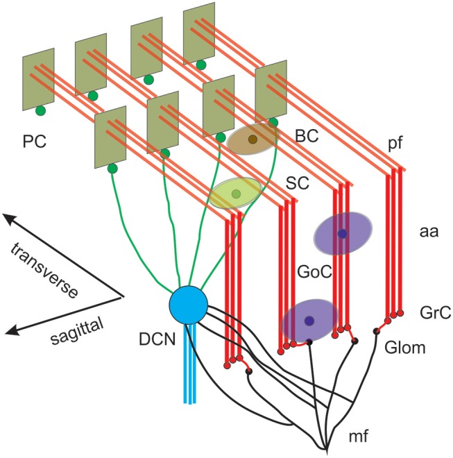
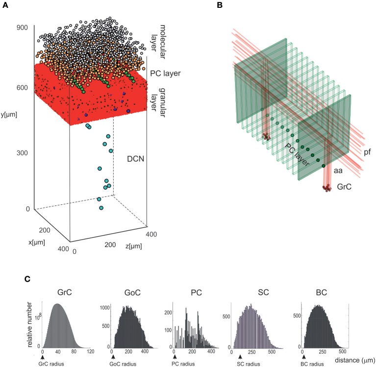
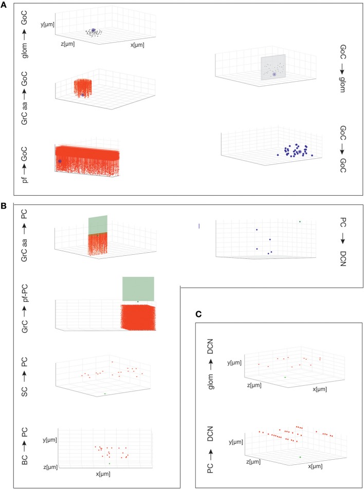
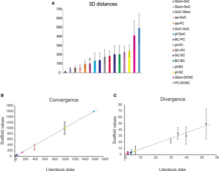
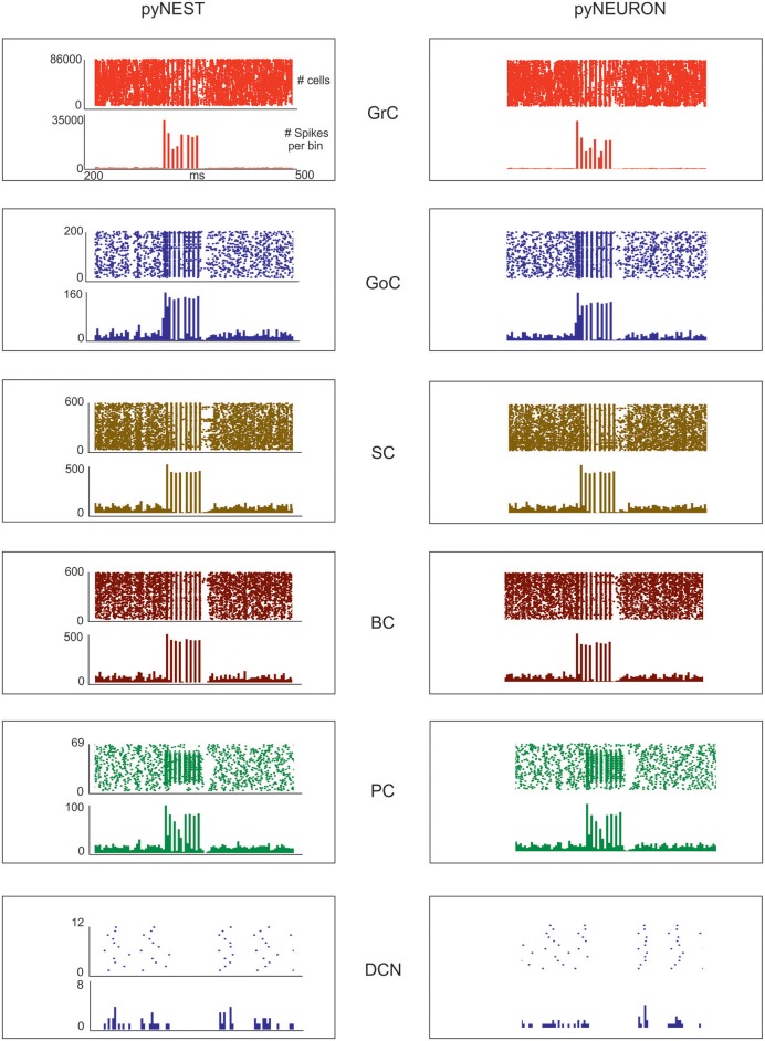
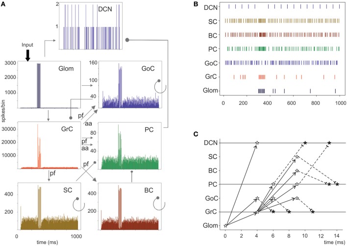
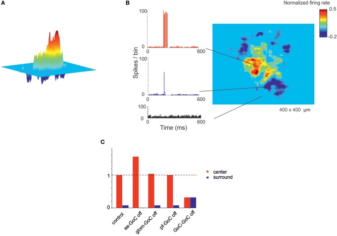
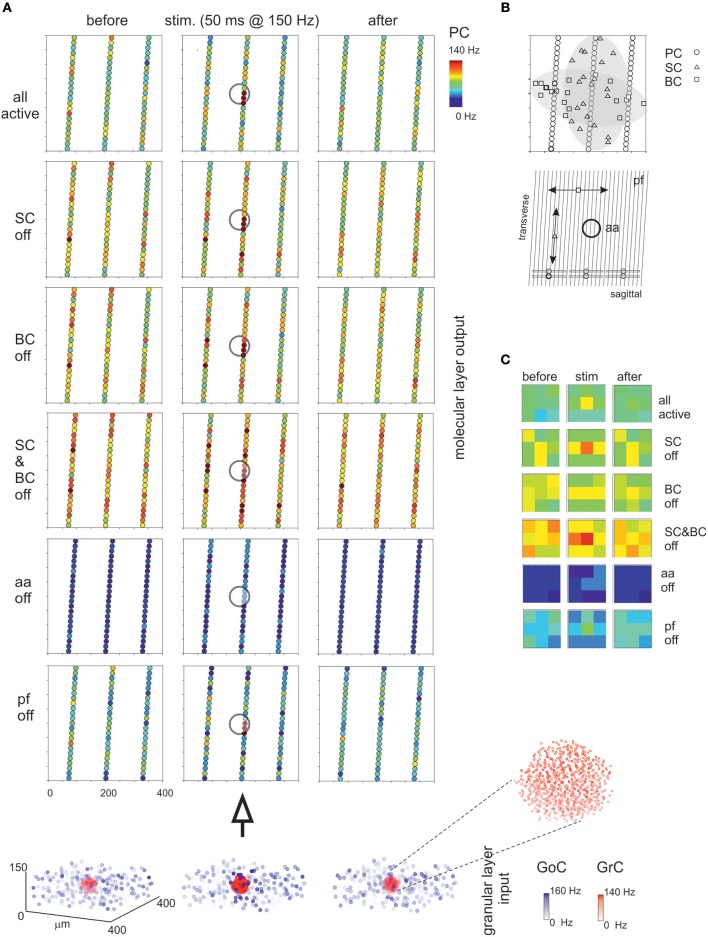
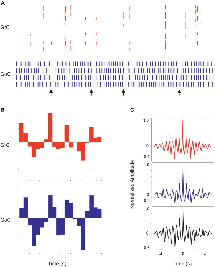
Reconstructing neuronal microcircuits through computational models is fundamental to simulate local neuronal dynamics. Here a scaffold model of the cerebellum has been developed in order to flexibly place neurons in space, connect them synaptically, and endow neurons and synapses with biologically-grounded mechanisms. The scaffold model can keep neuronal morphology separated from network connectivity, which can in turn be obtained from convergence/divergence ratios and axonal/dendritic field 3D geometries. We first tested the scaffold on the cerebellar microcircuit, which presents a challenging 3D organization, at the same time providing appropriate datasets to validate emerging network behaviors. The scaffold was designed to integrate the cerebellar cortex with deep cerebellar nuclei (DCN), including different neuronal types: Golgi cells, granule cells, Purkinje cells, stellate cells, basket cells, and DCN principal cells. Mossy fiber inputs were conveyed through the glomeruli. An anisotropic volume (0.077 mm³) of mouse cerebellum was reconstructed, in which point-neuron models were tuned toward the specific discharge properties of neurons and were connected by exponentially decaying excitatory and inhibitory synapses. Simulations using both pyNEST and pyNEURON showed the emergence of organized spatio-temporal patterns of neuronal activity similar to those revealed experimentally in response to background noise and burst stimulation of mossy fiber bundles. Different configurations of granular and molecular layer connectivity consistently modified neuronal activation patterns, revealing the importance of structural constraints for cerebellar network functioning. The scaffold provided thus an effective workflow accounting for the complex architecture of the cerebellar network. In principle, the scaffold can incorporate cellular mechanisms at multiple levels of detail and be tuned to test different structural and functional hypotheses. A future implementation using detailed 3D multi-compartment neuron models and dynamic synapses will be needed to investigate the impact of single neuron properties on network computation.

Keywords: Python; cerebellum; computational spiking models; connectome; pyNEST; pyNEURON.

Figure 1

Reconstruction of a scaffold model of the cerebellar network. Schematic representation of the cerebellar network (from D'Angelo et al., 2016). Glomeruli (Glom); mossy fiber (mf); Granule cells (GrC); ascending axon (aa); parallel fiber (pf); Golgi cells (GoC); stellate cell (SC); basket cell (BC); Purkinje cell (PC); Deep Cerebellar Nuclei cell (DCNC). Gloms transmit mf inputs to GrCs, which emit aa and pf, which in turn activate GoCs, PCs, SCs, and BCs. GoCs inhibit GrCs, SCs and BCs inhibit PCs. DCN cells are inhibited by PCs and activated by mf. Note the precise organization of PC dendrites, SC/BC dendrites and GoC dendritic arborization mainly on the parasagittal plane. The same abbreviations are used also in the following figures.

Figure 2

Cell placement and network architecture. (A) The cells are placed in the network 3D space using a Bounded Self-Avoiding Random Walk Algorithm. The figure shows the volume of 400 × 400 × 900 μm³ containing 96,737 neurons and 4,220,752 synapses used for simulations. (B) Projection of GrC axons to the molecular layer hosting the PCs (green dots in the PC layer are the somata, the thin green parallelepipeds above are the corresponding dendritic trees occupying the molecular layer). The figure shows two clusters of GrCs and the corresponding aa and pf, illustrating that the cerebellar network connectivity respects the 3D architecture shown in Figure 1. (C) Distributions of 3D pair-wise inter-soma distances within each neuronal population: GrCs, SCs, GoCs, BCs, and PCs. Note that the distributions are nearly normal, except for the PCs.

Figure 3

Cell connectivity: examples for specific connections. Examples of divergence and convergence at different connections in the cerebellar network space. The plots have base area (400 × 400 μm²) and thickness specific for each layer. The plots show a randomly selected pre-synaptic cell together with its connected post-synaptic neurons (divergence) or viceversa (convergence). (A) Connections of GrCs and GoCs. (B) Connections of PCs, SCs, and BCs. (C) Connections of DCNCs.

Figure 4

Cell connectivity: pair-wise distance prediction and convergence/divergence validation. (A) Pair-wise distance prediction deriving from the placement and subsequent cell-to-cell connectivity. The data that find correspondence in literature are indicated as asterisks. For each connection type, the pair-wise distances between connected cells (inter-soma distance) are reported. Data from: (1) (D'Angelo et al., 2013), (2) (Barmack and Yakhnitsa, 2008), (3) (Rieubland et al., 2014). (B,C) The plots compare divergence and convergence for the different connections of the scaffold with those anticipated experimentally. The regression lines show a very close correspondence of the model to experimental results. Linear regression lines are fitted to the data (divergence: r² = 0.98, slope = 0.88; convergence: r² = 0.99, slope = 0.99). Data from: (1) (Nieus et al., 2006), (2) (Dieudonne, 1998), (3) (D'Angelo et al., 2013), (4) (Solinas et al., 2010), (5) (Kanichay and Silver, 2008), (6) (Cesana et al., 2013), (7) (Hull and Regehr, 2012), (8) (Lennon et al., 2014), (9) (Huang et al., 2006), (10) (Jorntell et al., 2010), (11) (Sultan and Heck, 2003), (12) (Person and Raman, 2012), (13) (Boele et al., 2013).

Figure 5

Neuronal discharge. Raster plot and PSTH of the different neuron populations of the cerebellar network model in response to a mossy fiber burst (50 ms at 150 Hz on 2,932 gloms) superimposed on a 1 Hz random background. The two simulations used the same cerebellar scaffold and neurons, which were translated from pyNEST into pyNEURON. The basal activity of the different cell populations is visible before and after the stimulus. The Glom patterns at the input are imposed, so they are identical for both simulations. The mean population firing rates for GrCs are similar between the two simulations, probably due to the very high number of GrCs. Minor differences are detectable for the other neuron types.

Figure 6

Cerebellar network response to a mossy fiber burst. (A) Spikegrams of all cerebellar neurons in the model. A burst in gloms causes a burst-to-burst propagation in GrCs and PCs. GoCs, SCs, and BCs also generate bursts that, by being inhibitory, contribute to terminate the GrC, and PC bursts and to generate the burst-pause PC response. The DCN cells show a pause during stimulation. (B) Raster plot of one cerebellar neuron for each population in the model. Note the spread of the mf bursts inside the cerebellar cortical networks and the corresponding pause in the DCN. (C) Spike-time response plot showing the temporal sequence of neuronal activation and inhibition. The arrows represent the connectivity (solid lines show excitatory connections, dashed lines inhibitory connections). The stars represent the post-synaptic neuron response: white stars are excited neurons, black stars are inhibited neurons.

Figure 7

Center-surround organization of activity in the granular layer. (A) In response to a mossy fiber burst (40 gloms at 150 Hz for 50 ms), the granular layer responds with a core (red area) of activity surrounded by inhibition (blue area). (B) PSTH of GrCs in the center-surround. The activity in the core is characterized by robust spike bursts, while just sporadic spikes are generated in the surround. No activity changes are observed outside the center-surround structure. (C) The histogram shows the changes in center-surround extension that occur following selective switch-off of synapses impinging on GoCs. Note the prominent role of aa-GoC synapses and GoC-GoC synapses (bars are values normalized to control).

Figure 8

Maps of PC activation and sensitivity to molecular layer connectivity. (A) The maps show the activity change of PCs in response to a mossy fiber burst (40 glom at 150 Hz for 50 ms). The pattern of activity is determined by various connection properties that are tested in turn. (all active) PC inhibition is achieved through a differential orientation of SC axons (mostly transversal or “on-beam”) vs. BC axons (mostly sagittal or “off-beam”) and that PC excitation depends on both aa and pf synapses with specific origin from GrCs. Alternative patterns are generated by (SC off) the specific switch-off of SC, (BC off) the specific switch-off of BC, or (SC&BC off) the complete switch-off of both SC and BC, (aa off) the specific switch-off of aa synapses, (pf off) the specific switch-off of pf synapses. It should be noted that these changes in network connectivity modify the PC discharge patterns both on-beam and off-beam and extend to a distance that reflects the propagation of activity through the molecular layer interneuron network. The circles indicate the location of the underlying active spots of activity in the granular layer. The bottom plot represents the activity of GoCs (blue) and GrCs (red) before, during and after the stimulus burst. This activity occurs in a spot (enlarged in the inset) corresponding to the center-surround shown in Figure 7. (B) The schematic diagrams show the orientation of fibers and connections in the network. (C) The PC activity was averaged into 3 × 3 matrices in order to better appreciate where activity changes take place. Note the emergence of the central spot in several cases.

Figure 9

Coherent low-frequency oscillations in granular layer neurons. Activity of GrCs (red) and GoCs (blue) during sustained 5 Hz random mf input. (A) Raster plots from exemplar GrCs and GoCs. Note that synchronous patterns are visible in the neuronal response (arrows). In this regimen, GoC activity is more intense than GrC activity due to the autorhytmic discharge of GoC neurons. The neurons are not necessarily part of a center-surround and therefore not all activities appear correlated. (B) Cumulative PSTH of the whole GrC and GoC populations of the model along a 5 s period. Note that the two PSTH show marked low-frequency oscillations (average 1.8 Hz) around their average level of activity. (C) Autocorrelograms of activity in the GrC and GoC populations and crosscorrelogram of the GrC and GoC populations (in this example the inhibition among GoCs is switched off). Note the high level of correlation in all the three cases on the same main frequency of 1.8 Hz.

References

1. Aizenman C. D., Huang E. J., Linden D. J. (2003). Morphological correlates of intrinsic electrical excitability in neurons of the deep cerebellar nuclei. J. Neurophysiol. 89, 1738–1747. 10.1152/jn.01043.2002 - DOI - PubMed
1. Akram M. A., Nanda S., Maraver P., Armananzas R., Ascoli G. A. (2018). An open repository for single-cell reconstructions of the brain forest. Sci. Data 5:180006. 10.1038/sdata.2018.6 - DOI - PMC - PubMed
1. Barbour B. (1993). Synaptic currents evoked in Purkinje cells by stimulating individual granule cells. Neuron 11, 759–769. 10.1016/0896-6273(93)90085-6 - DOI - PubMed
1. Barmack N. H., Yakhnitsa V. (2008). Functions of interneurons in mouse cerebellum. J. Neurosci. 28, 1140–1152. 10.1523/JNEUROSCI.3942-07.2008 - DOI - PMC - PubMed
1. Billings G., Piasini E., Lorincz A., Nusser Z., Silver R. A. (2014). Network structure within the cerebellar input layer enables lossless sparse encoding. Neuron 83, 960–974. 10.1016/j.neuron.2014.07.020 - DOI - PMC - PubMed