Single particle cryo-EM reconstruction of 52 kDa streptavidin at 3.2 Angstrom resolution

Abstract

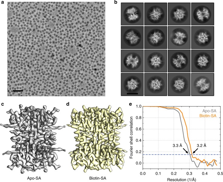
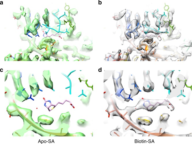
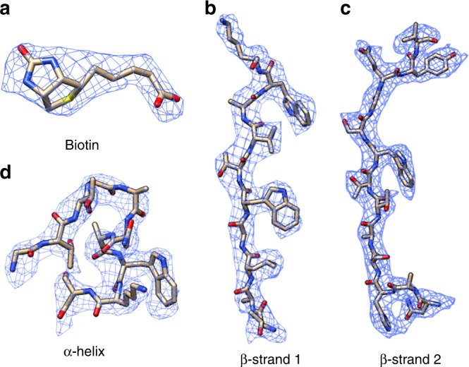
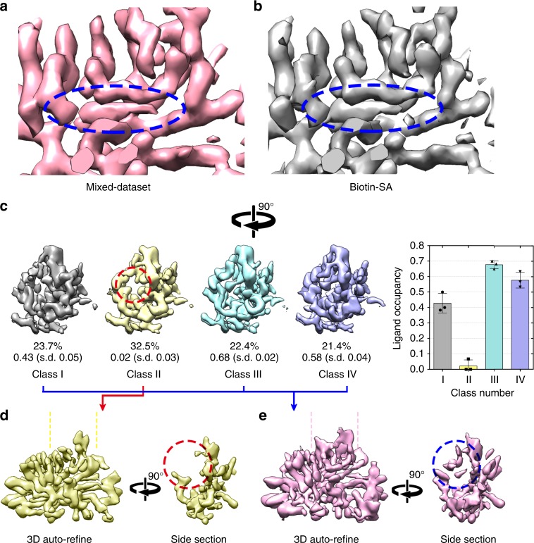
The fast development of single-particle cryogenic electron microscopy (cryo-EM) has made it more feasible to obtain the 3D structure of well-behaved macromolecules with a molecular weight higher than 300 kDa at ~3 Å resolution. However, it remains a challenge to obtain the high-resolution structures of molecules smaller than 200 kDa using single-particle cryo-EM. In this work, we apply the Cs-corrector-VPP-coupled cryo-EM to study the 52 kDa streptavidin (SA) protein supported on a thin layer of graphene and embedded in vitreous ice. We are able to solve both the apo-SA and biotin-bound SA structures at near-atomic resolution using single-particle cryo-EM. We demonstrate that the method has the potential to determine the structures of molecules as small as 39 kDa.

Fig. 1

The SPA cryo-EM of SA. a A representative micrograph of the SA specimen by the VPP-Cs-corrector-coupled cryo-EM. The scale bar represents 20 nm. b Representative 2D class averages of SA particle images. The scale bar represents 5 nm. c The 3D reconstruction of apo-SA at 3.3 Å resolution from 23,991 particles and d the 3D reconstruction of the biotin-bound SA at 3.2 Å resolution from 45,686 particles. e The fourier shell correlation (FSC) curves of the two reconstructions using the gold-standard criteria

Fig. 2

Comparison between the reconstructions of the two SA states. a, c The region around the biotin-binding pocket of the apo-SA EM map has an empty density of the pocket and a missing loop 46–51 density, whereas in b, d the biotin-bound SA EM map, these two densities are well resolved with the atomic model of the biotin ligand and the loop 46–51

Fig. 3

Biotin-SA local maps with their corresponding atomic models. a Biotin density in the binding pocket. b Representative densities of secondary structures: β-sheet (b, c) and α-helix (d)

Fig. 4

Reconstruction and classification using the mixed dataset. a The 3D reconstruction of the mixed dataset (apo-SA + biotin-SA) with 3.1 Å resolution demonstrates a biotin-bound-like density (circled in blue) as b the 3D reconstruction of biotin-SA at 3.2 Å resolution of a monomer. c Asymmetric 3D classification reconstructions of the mixed dataset. The empty density of the biotin-binding pocket in the monomer of the Class II reconstruction is circled in red in contrast to the ligand densities in the other classes. The percentage of particles and ligand occupancy in each class are labeled. A column graph with error bars to show the ligand occupancy of each class is shown. The 3D reconstruction of d class II and e the merged class I–III–IV indicated the apo-SA and biotin-SA individually. A side section comparison demonstrated the extra density of loop 46–51 and the biotin molecule in e (blue circle). Error bars (SD) were calculated from three random repeats. Source data are provided as a Source Data file

Fig. 5

Reconstructions of subtracted SA in different oligomeric states. a The diagrammatic sketch of the subtraction in raw biotin-SA particles. The white parts were subtracted from the individual particle images based on related angular information, with the blue part left for image processing (monomer, dimer, and trimer from left to right). b 2D classification results from subtracted datasets in different oligomeric states either using the angular information generated from the 3D refinement of the SA tetramers (Skip Align) or omitting the angular information in a reference-free mode (Search Align). The scale bar represents 5 nm. c 3D reconstructions with local angular search of the three subtracted datasets. The initial rough angular information was generated from the 3D refinement of the SA tetramers. d 3D reconstructions with global angular search. The results indicate that only the trimeric dataset could yield a successful global refinement from scratch

Fig. 6

SA particles on graphene–water and air–water interfaces. a The X–Y cross-section corresponding to the graphene–water interface (GWI) from a reconstructed tomogram. The uneven distribution of particles is indicated as a clustering area (red arrow) and lacuna area (blue arrow). The scale bar represents 100 nm. b The X–Y cross-section corresponding to the air–water interface (AWI) from the same reconstructed tomogram as in a. c A micrograph containing a clustering area (red arrow) and uniform distribution area (blue arrow). The boundaries of the two areas are marked by dashed lines. The scale bar represents 20 nm. d The same micrograph as in c, with the particles that contributed to the final high-resolution reconstruction circled in green. e The numbers of particles in Subset A and Subset B after the 2D Classification (After2D), after the first 3D Classification (After3D), and in the final Refinement (Final Refine) were counted in 749 selected micrographs with a clear clustering feature. f The percentages of particles from Subset A and Subset B in the different data processing steps. g The distribution of the major particle orientations, top view (rounded-like) and side view (butterfly-like), in Subset A and Subset B, respectively. The particles in Subset B demonstrated a severe preferential orientation. Source data are provided as a Source Data file

References

1. Cheng Y, Grigorieff N, Penczek PA, Walz T. A primer to single-particle cryo-electron microscopy. Cell. 2015;161:438–449. doi: 10.1016/j.cell.2015.03.050. - DOI - PMC - PubMed
1. Bai XC, McMullan G, Scheres SH. How cryo-EM is revolutionizing structural biology. Trends Biochem. Sci. 2015;40:49–57. doi: 10.1016/j.tibs.2014.10.005. - DOI - PubMed
1. Glaeser RM. How good can cryo-EM become? Nat. Methods. 2015;13:28. doi: 10.1038/nmeth.3695. - DOI - PubMed
1. Li X, et al. Electron counting and beam-induced motion correction enable near-atomic-resolution single-particle cryo-EM. Nat. Methods. 2013;10:584. doi: 10.1038/nmeth.2472. - DOI - PMC - PubMed
1. Scheres SHW. RELION: implementation of a Bayesian approach to cryo-EM structure determination. J. Struct. Biol. 2012;180:519–530. doi: 10.1016/j.jsb.2012.09.006. - DOI - PMC - PubMed
Publication types