Observations and Projections of Heat Waves in South America

Abstract

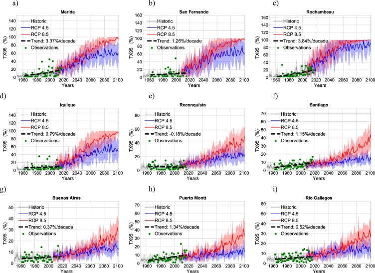
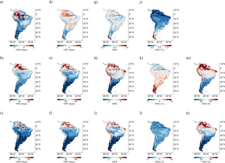
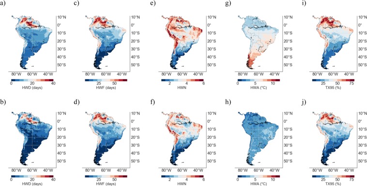
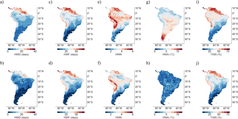
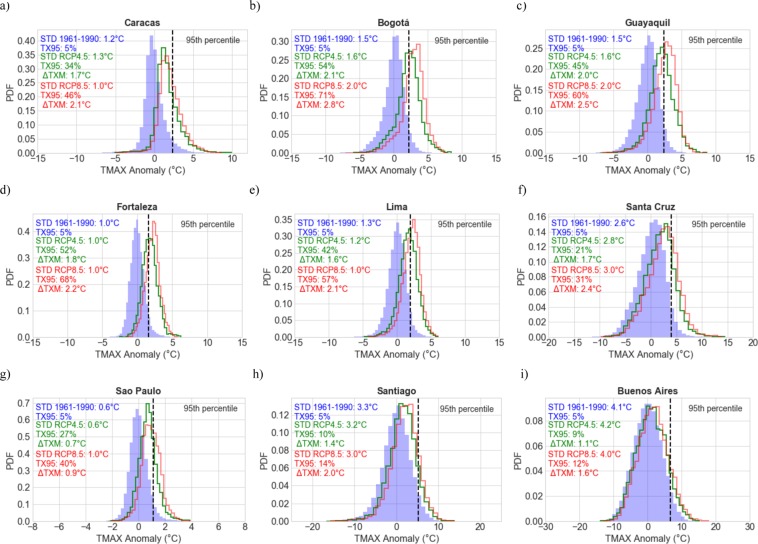
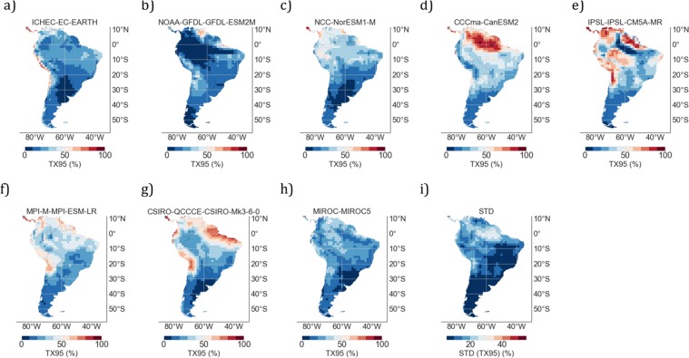
Although Heat Waves (HWs) are expected to increase due to global warming, they are a regional phenomenon that demands for local analyses. In this paper, we assess four HW metrics (HW duration, HW frequency, HW amplitude, and number of HWs per season) as well as the share of extremely warm days (TX95, according to the 95th percentile) in South America (SA). Our analysis included observations as well as simulations from global and regional models. In particular, Regional Climate Models (RCMs) from the Coordinated Regional Climate Downscaling Experiment (CORDEX), and Global Climate Models (GCMs) from the Coupled Model Intercomparison Project Phase 5 (CMIP5) were used to project both TX95 estimates and HW metrics according to two representative concentration pathways (RCP4.5 and RCP8.5). We found that in recent decades the share of extremely warm days has at least doubled over the period December-January-February (DJF) in northern SA; less significant increases have been observed in southern SA. We also found that by midcentury, under the RCP4.5 scenario, extremely warm DJF days (as well as the number of HWs per season) are expected to increase by 5-10 times at locations close to the Equator and in the Atacama Desert. Increases are expected to be less pronounced in southern SA. Projections under the RCP8.5 scenario are more striking, particularly in tropical areas where half or more of the days could be extremely warm by midcentury.

Figure 1

Locations of weather stations considered in this study (see blue dots). RCM simulations were used to project TX95 values and HW metrics for future climate scenarios (RCP4.5 and RCP 8.5) for 9 major cities (see yellow dots). The elevation map was created using the CGIAR-CSI SRTM dataset. Plot was generated by using Python’s Matplotlib Library.

Figure 2

Share of extremely warm DJF days (TX95) from observations over the period 1961–2016 (green dots), from historical RCM simulations over the period 1951–2005 (gray line), and from RCM projections over the period 2005–2100 (blue line for RCP4.5; red line for RCP8.5). TX95 values correspond to the percentage of DJF days exceeding the 95th percentile of the T_MAX anomaly distribution corresponding to the base period. The trend line (as well as the decadal trend computed using observations over the period 1961–2016) is also shown in each plot. (a) Merida; (b) San Fernando; (c) Rochambeau; (d) Iquique; (e) Reconquista; (f) Santiago; (g) Buenos Aires; (h) Puerto Montt; (i) Rio Gallegos. Plots were generated by using Python’s Matplotlib Library.

Figure 3

Multi-Model-Mean (MMM) of HW metrics from RCM simulations over the period 1961–1990 (1^st row); TX95 estimates over the base period 1961–1990 are not shown since they were by definition 5%. MMM of HW metrics and TX95 estimates from RCM simulations over the period 2046–2055 under the RCP4.5 scenario (2^nd row). Change, 1961–1990 to 2046–2055 (RCP4.5), in TX95 estimates and in HW metrics (3^nd row). (a–c) HWD; (d–f) HWF; (g–i) HWN; (j–l) HWA; and (m,n) TX95. Plots were generated by using Python’s Matplotlib Library.

Figure 4

Multi-Model-Mean (MMM) of HW metrics and TX95 estimates from RCM simulations over the period 2090–2100 under the RCP4.5 scenario (1^st row). Change, 1961–1990 to 2090–2100 (RCP4.5), in HW metrics and in TX95 estimates (2^nd row). (a,b) HWD; (c,d) HWF; (e,f) HWN; (g,h) HWA; and (i,j) TX95. Plots were generated by using Python’s Matplotlib Library.

Figure 5

Multi-Model-Mean (MMM) of HW metrics from GCM simulations over the period 1961–1990 (1^st row); TX95 estimates over the base period 1961–1990 are not shown since they were by definition 5%. MMM of HW metrics and TX95 estimates from GCM simulations over the period 2046–2055 under the RCP4.5 scenario (2^nd row). Change, 1961–1990 to 2046–2055 (RCP4.5), in TX95 estimates and in HW metrics (3^nd row). (a–c) HWD; (d–f) HWF; (g–i) HWN; (j–l) HWA; and (m,n) TX95. Plots were generated by using Python’s Matplotlib Library.

Figure 6

Multi-Model-Mean (MMM) of TX95 estimates and HW metrics computed from GCM simulations over the period 2090–2100 under the RCP4.5 scenario (1^st row). Change, 1961–1990 to 2090–2100 (RCP4.5), in TX95 estimates and in HW metrics (2^nd row). (a,b) HWD; (c,d) HWF; (e,f) HWN; (g,h) HWA; and (i,j) TX95. Plots were generated by using Python’s Matplotlib Library.

Figure 7

Histograms of the daily DJF T_MAX anomalies rendered by the RCMs over the base period 1961–1990 (blue histograms) as well as over the period 2046–2055 (green histograms for RCP 4.5; red histograms for RCP8.5). (a) Caracas; (b) Bogotá; (c) Guayaquil; (d) Fortaleza; (e) Lima; (f) Santa Cruz; (g) Sao Paulo; (h) Santiago; (i) Buenos Aires. The dotted vertical line in each plot indicates the 95th percentile of the T_MAX anomaly distribution corresponding to the base period. Also shown in the upper left corner of each plot and for each histogram: the standard deviation (STD); the share of extremely warm DJF days (TX95); and the shift in the mean (TXM), 1961–1990 to 2046–2055, of the DJF T_MAX anomalies. Plots were generated by using Python’s Matplotlib Library.

Figure 8

TX95 estimates by midcentury (2046–2055) computed from different RCMs: (a) ICHEC-EC-EARTH; (b) NOAA-GFDL-GFDL-ESM2M; (c) NCC-NorESM1-M; (d) CCCma-CanESM2; (e) IPSL-IPSL-CM5A-MR; (f) MPI-M-MPI-ESM-LR; (g) CSIRO-QCCCE-CSIRO-Mk3-6-0; (h) MIROC-MIROC5; (i) ECMWF-ERAINT- MPI-M-MPI-ESM-LR; (j) Standard deviation (STD) computed by using the spread of decadal TX95 estimates (2046–2055) from different RCMs (see plots a–i). In this figure, RCMs in plot 8f and in 8i were driven by the same GCM (MPI-M-MPI-ESM-LR; see plot 9f). Plots were generated by using Python’s Matplotlib Library.

Figure 9

TX95 estimates by midcentury (2046–2055) computed from different GCMs: (a) ICHEC-EC-EARTH; (b) NOAA-GFDL-GFDL-ESM2M; (c) NCC-NorESM1-M; (d) CCCma-CanESM2; (e) IPSL-IPSL-CM5A-MR; (f) MPI-M-MPI-ESM-LR; (g) CSIRO-QCCCE-CSIRO-Mk3-6-0; (h) MIROC-MIROC5; (i) Standard deviation (STD) computed by using the spread of decadal TX95 estimates (2046–2055) from different GCMs (see plots a–h). Plots were generated by using Python’s Matplotlib Library.

References

1. Perkins SE. A review on the scientific understanding of heatwaves—Their measurement, driving mechanisms, and changes at the global scale. Atmos. Res. 2015;164:242–267. doi: 10.1016/j.atmosres.2015.05.014. - DOI
1. Smith A, Lott N, Vose R. The integrated surface database: Recent developments and partnerships. Bull. Am. Meteorol. Soc. 2011;92:704–708. doi: 10.1175/2011BAMS3015.1. - DOI
1. Perkins SE, Alexander LV. On the measurement of heat waves. J. Clim. 2013;26:4500–4517. doi: 10.1175/JCLI-D-12-00383.1. - DOI
1. Perkins SE, Alexander LV, Nairn JR. Increasing frequency, intensity and duration of observed global heatwaves and warm spells. Geophys. Res. Lett. 2012;39:L20714.
1. Ragone F, Wouters J, Bouchet F. Computation of extreme heat waves in climate models using a large deviation algorithm. Proc. Natl. Acad. Sci. USA. 2018;115:24–29. doi: 10.1073/pnas.1712645115. - DOI - PMC - PubMed
Publication types