Hydrothermal vents trigger massive phytoplankton blooms in the Southern Ocean

Abstract

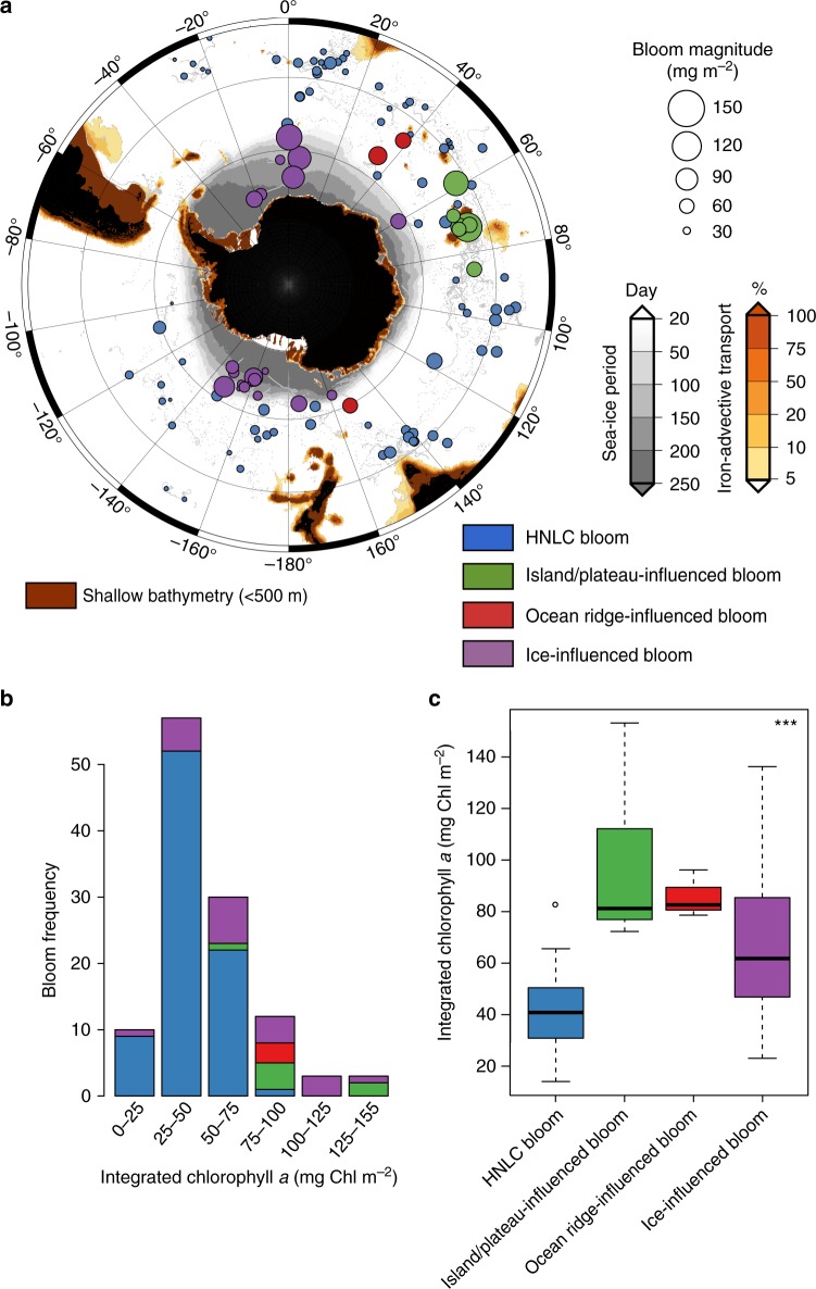
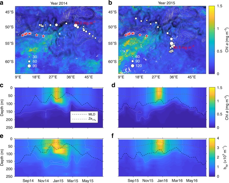
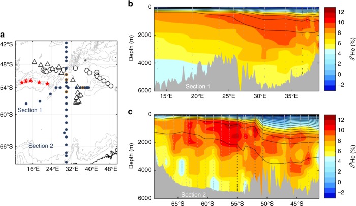
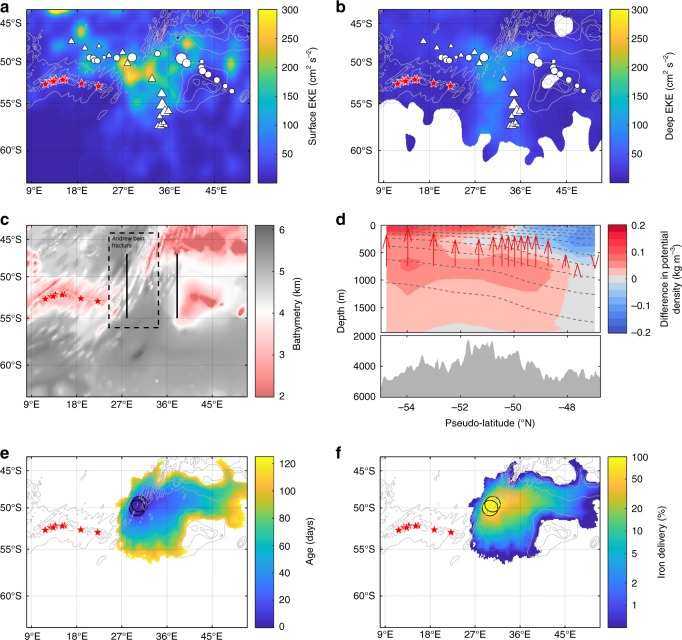
Hydrothermal activity is significant in regulating the dynamics of trace elements in the ocean. Biogeochemical models suggest that hydrothermal iron might play an important role in the iron-depleted Southern Ocean by enhancing the biological pump. However, the ability of this mechanism to affect large-scale biogeochemistry and the pathways by which hydrothermal iron reach the surface layer have not been observationally constrained. Here we present the first observational evidence of upwelled hydrothermally influenced deep waters stimulating massive phytoplankton blooms in the Southern Ocean. Captured by profiling floats, two blooms were observed in the vicinity of the Antarctic Circumpolar Current, downstream of active hydrothermal vents along the Southwest Indian Ridge. These hotspots of biological activity are supported by mixing of hydrothermally sourced iron stimulated by flow-topography interactions. Such findings reveal the important role of hydrothermal vents on surface biogeochemistry, potentially fueling local hotspot sinks for atmospheric CO₂ by enhancing the biological pump.

Fig. 1

Phytoplankton bloom distribution, type and biomass in the Southern Ocean. Map (a) of the different bloom types (i.e., blue circles: HNLC; green circle: island/plateau-influenced; red circle: ocean ridge-influenced; purple circle: ice-influenced) sampled. The magnitude of the bloom (i.e., the maximum depth-integrated biomass) is related to the size of the colored circles. The gray dots indicate the individual float profiles. The red, orange, and gray zones are, respectively, shallow areas (>500 m), areas with downstream iron delivery (%; percent of iron remaining in a water parcel after scavenging relative to its initial concentration in shallow areas based on the Lagrangian modeling of horizontal iron delivery), and areas characterized by a seasonal sea ice cover. Histograms (b) of the frequency of and boxplot (c) according to the bloom type are displayed in relation to the bloom magnitude. In c, the top and bottom limits of each box are the 25th and 75th percentiles, respectively. The lines extending above and below each box, i.e., whiskers, represent the full range of non-outlier observations for each variable beyond the quartile range. The results of the Kruskal–Wallis H test are shown in panel c and depict regions with statistically significant differences between the magnitudes of the bloom at the 95 % level (p < 0.05). Asterisks (***) denote highly significant results (p < 0.0001)

Fig. 2

Massive phytoplankton blooms stimulated by upwelled hydrothermally influenced deep waters along the Southwest Indian Ridge (SWIR). Maps (a and b)of the SWIR in the Indian sector of the Southern Ocean and float trajectories. The maximum depth-integrated biomass (mg Chl m⁻²) is depicted according the size of the circles. Satellite-derived surface chlorophyll a climatologies (8-days GLOBcolour composite products) were retrieved from November to January a 2014–2015 and b 2015–2016. Black arrows correspond to altimetry-derived geostrophic velocities (AVISO MADT daily product) averaged over the same period. Gray lines represent the 2000, 3000 and 4000 isobaths. Time series of the 0–250 m vertical distribution of chlorophyll a (c and d) and backscattering (e and f) for the two BGC-Argo floats (WMO 6901585 and 2902130). The black and gray dashed lines are, respectively, representing the mixed layer depth (determined by a density-derived method with a density threshold of 0.03 kg m⁻³) and the euphotic zone depth (defined as the depth of 1% of surface irradiance according Morel et al.; Eq. 10). The red stars indicate the position of hydrothermal vents from Tao et al.

Fig. 3

Hydrothermally influenced deep waters along the SWIR. Map (a) showing the locations of the bathymetry of the SWIR (contour levels: 2000, 3000, and 4000 m), the hydrothermal vents (red stars), the two BGC-Argo floats (black triangle dots: float WMO 6901585 and black circle dots: float WMO 2902130), and of the two sections (filled blue circle dots; b and c) of interpolated δ³He. Note that all the vertical δ³He profiles, where the surface eddy kinetic energy is high (EKE; >150 cm² s⁻²), have been highlighted by additional orange circle dots in a and by darker gray in b and c

Fig. 4

Topographically upwelled waters in the vicinity of the Antarctic Circumpolar Current along the SWIR. Maps of the eddy kinetic energy (EKE) at the surface (a) and at depth (b, approximately 1000 meters). The surface EKE was derived from altimetry-derived velocities (AVISO MADT daily product) over the 2003–2017 period. The deep EKE was calculated from the Argo-derived velocities during their parking depth and available in the ANDRO dataset (2000–2016). The maximum depth-integrated biomass (mg Chl a m⁻²) is also depicted according the size of the dots (triangle: float WMO 6901585 and circle: float WMO 2902130). c Maps of bathymetry of the SWIR, the Andrew Bain fracture zone (as indicated by the dashed box; http://www.marineregions.org/gazetteer.php?p=details&id=7253) and the two meridional sections at 28°E and 38°E (between latitude 47°–55°S; plain black lines) where the difference in potential density Δσ shown in panel d was determined. d Climatological difference of potential density, Δσ, between the two meridional sections at 38°E and 28°E in the upper 2000 m (between latitude 47°–55°S). Gray shading represents the mean bottom topography between 28 and 38°E, and the red arrows are provided to show the sense of downstream isopycnal adjustment at 750-m depth. The difference in Δσ is an alongstream difference across the two sections, which is converted back to latitude for ease of reading (therefore referred to as pseudo-latitude). See the Methods for more details. e–f Satellite altimetry-derived Lagrangian modeling of the iron pathways from the departure of the SWIR as shown in e age (days since having left the SWIR) and in f iron delivery. Black circles in e–f indicate the origin of the iron pathways in the surface layer. The red stars in a–c, e and f are related to the position of hydrothermal vents from Tao et al.. The continuous and dashed gray lines indicate, respectively, the bathymetry (a, b, e and f) of the SWIR (contour levels: 2000, 3000, and 4000 m) and the isopycnals (d)

References

1. Moore JK, Doney SC, Glover DM, Fung IY. Iron cycling and nutrient-limitation patterns in surface waters of the World Ocean. Deep Sea Res. 2001;2 49:463–507. doi: 10.1016/S0967-0645(01)00109-6. - DOI
1. Tagliabue A, et al. The integral role of iron in ocean biogeochemistry. Nature. 2017;543:51–59. doi: 10.1038/nature21058. - DOI - PubMed
1. Boyd PW, Ellwood MJ. The biogeochemical cycle of iron in the ocean. Nat. Geosci. 2010;3:675. doi: 10.1038/ngeo964. - DOI
1. Tagliabue A, et al. Hydrothermal contribution to the oceanic dissolved iron inventory. Nat. Geosci. 2010;3:252–256. doi: 10.1038/ngeo818. - DOI
1. Tagliabue A, Aumont O, Bopp L. The impact of different external sources of iron on the global carbon cycle. Geophys. Res. Lett. 2014;41:920–926. doi: 10.1002/2013GL059059. - DOI
Publication types