Heterochromatin drives compartmentalization of inverted and conventional nuclei

Abstract

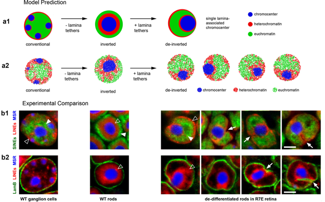
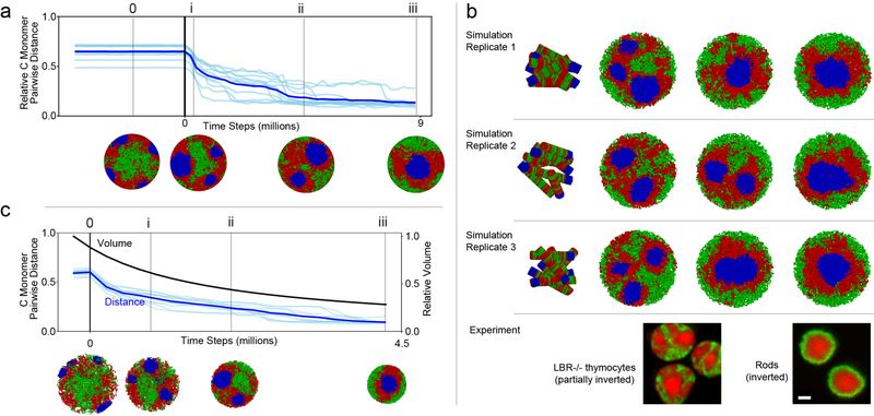
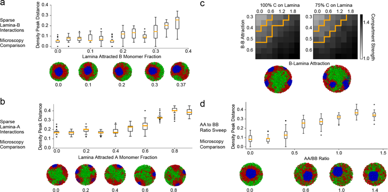
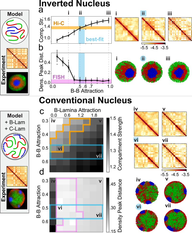
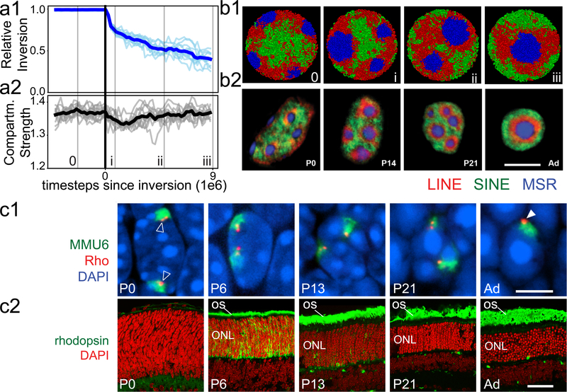
The nucleus of mammalian cells displays a distinct spatial segregation of active euchromatic and inactive heterochromatic regions of the genome^1,2. In conventional nuclei, microscopy shows that euchromatin is localized in the nuclear interior and heterochromatin at the nuclear periphery^1,2. Genome-wide chromosome conformation capture (Hi-C) analyses show this segregation as a plaid pattern of contact enrichment within euchromatin and heterochromatin compartments³, and depletion between them. Many mechanisms for the formation of compartments have been proposed, such as attraction of heterochromatin to the nuclear lamina^2,4, preferential attraction of similar chromatin to each other^1,4-12, higher levels of chromatin mobility in active chromatin^13-15 and transcription-related clustering of euchromatin^16,17. However, these hypotheses have remained inconclusive, owing to the difficulty of disentangling intra-chromatin and chromatin-lamina interactions in conventional nuclei¹⁸. The marked reorganization of interphase chromosomes in the inverted nuclei of rods in nocturnal mammals^19,20 provides an opportunity to elucidate the mechanisms that underlie spatial compartmentalization. Here we combine Hi-C analysis of inverted rod nuclei with microscopy and polymer simulations. We find that attractions between heterochromatic regions are crucial for establishing both compartmentalization and the concentric shells of pericentromeric heterochromatin, facultative heterochromatin and euchromatin in the inverted nucleus. When interactions between heterochromatin and the lamina are added, the same model recreates the conventional nuclear organization. In addition, our models allow us to rule out mechanisms of compartmentalization that involve strong euchromatin interactions. Together, our experiments and modelling suggest that attractions between heterochromatic regions are essential for the phase separation of the active and inactive genome in inverted and conventional nuclei, whereas interactions of the chromatin with the lamina are necessary to build the conventional architecture from these segregated phases.

Extended Data Figure 1.. Hi-C replicates show reproducible features.

Hi-C maps are qualitatively similar between replicates. Hi-C maps (plotted log₁₀) for an 87 MB region of chromosome 1; compartment profiles indicating regions in the A (green) and B (red-brown) compartments are shown above. Full maps are available to browse on HiGlass (http://higlass.io/app/?config=JLOhiPILTmq6qDRicHMJqg). For quantitative comparison, see ED Figs 3, 4, and 5.

Extended Data Figure 2.. The majority of thymocytes are actively cycling cells in both WT (left column) and LBR-null (right column) mice

Thymus cryosections are immunostained with antibodies for Ki67, a marker of cycling cells, and for phosphorylated H3S10, a marker for G2 and mitotic cells. Note, that in agreement with a seemingly normal immune system of LBR-null mice, the number of cycling thymocytes in their thymuses is comparable to that of WT mice. M, mitotic cells; G2, cells in mid/late G2. Ki67 staining: projections of 5 μm confocal stacks. H3S10ph staining: projections of 10 μm (for overviews) or 3 μm (for zoomed areas) confocal stacks. Antibodies: mouse anti-H3S10ph (Abcam, ab14955) and rabbit anti-Ki67 (Abcam, ab15580). Immunostaining and microscopy were performed as described in Methods.

Extended Data Figure 3.. Quantitative analysis of TADs.

a, Average TADs, based on domain calls from ESC (embryonic stem cells). Ticks indicate start and end of TADs. The visual suggestion is that TADs are weakest in rods and strongest in non-rod neurons, with the thymocytes intermediate. b, TAD strength is weakest in rods and strongest in non-rod neurons. TAD strength is the ratio of average contacts within the TAD (pink triangle on the inset) to average contacts between TADs (blue triangles). TAD strength is calculated separately for each autosome in two replicas. (n=38 chromosomes, centerline is median, box is between lower and upper quartiles, whiskers extend to 1.5 times the interquartile range). c, Spearman correlation of insulation profiles across multiple mouse cell types (data from references^,, first author indicated in row/column label, GEO accession numbers GSE35156, GSE63525), clustered hierarchically. d, Average insulation profile (Methods) around TAD boundaries called in ESC. The minimum insulation score of each profile is set to zero. We symmeterize noise by reflecting around the TAD boundary and averaging the reflected and original profiles. e, Decay of contact probability, P(s), as a function of genomic separation, s. Shaded areas are bounded by P(s) curves for biological replicas. All P(s) curves are normalized to their value at 10kb. For rods, the steeper slope below 1Mb and lack of a rollover in contrast to the other three cell types is indicative of weaker TADs, as in Schwarzer et al. f, TAD strength as a function of cell type (columns) and cell type from which TADs are called (rows) (data from references^,,, first author indicated in row/column label, GEO accession numbers GSE98671, GSE63525, GSE93431). Note that rods cluster with cell types with demonstrated weaker TADs. TAD strength is computed differently than in ED Fig. 3b (Methods). g, Average insulation profile (Methods) oriented around top 10⁴ scoring CTCF motifs. For scoring, we used the FIMO algorithm, with a position weight matrix for the M1 motif as in Schmidt et al. The minimum insulation score of each profile is set to zero, and the CTCF motif points to the left. This provides a TAD-call independent method of inferring TAD strength, given that CTCF is frequently present at the borders of TADs. h, Snapshot of Hi-Glass view of the four data sets, close to the diagonal (chr12:77,538,523–85,180,785 & chr12:79,240,367–82,837,977, 32kb resolution). Rods are almost completely lacking TADs and non-rod neurons have very strong TADs, upon inspection. Datasets can be browsed in a more in-depth fashion on a public server (http://higlass.io/app/?config=JLOhiPILTmq6qDRicHMJqg)

Extended Data Figure 4.. Quantitative analysis of territories.

a, Hi-C contact maps for chromosomes 1, 2, and 3 show both a checkerboard pattern in cis (within a chromosome) and trans (between chromosomes), reflecting compartmentalization, and more frequent cis than trans contacts, reflecting chromosome territoriality. Views are shown for the second biological replicate, binned at 500kb. b, Average number of contacts between pairs of chromosomes. Average cis contacts are much higher than trans contacts. Maps are normalized by their sums. c, Average contacts in trans. For every unique pair of chromosomes, we average the first 60Mb, binned at 500kb resolution. Maps are normalized to their means, and plotted in log-space. There is evidence of weak enrichment among chromocenter-proximal regions in trans, independent of inversion status. d, Consistent with the low cis contact fraction revealed by Hi-C, chromosome 11 visualized by FISH (green) has a more diffuse territory in postmitotic rods and non-rod neurons in comparison to cycling thymocytes of both genotypes. Projections of 2 μm confocal stacks; scale bars, 5 μm. The chromosome painting was performed in four independent experiments. e, Chromosome territoriality, measured as the ratio of cis contacts to cis+trans contacts, is weaker in rods and non-rod neurons in comparison to conventional and inverted thymocytes. The schematic illustrates the compared regions. i, Scatterplot of compartmentalization and territoriality. The two metrics are not necessarily related.

Extended Data Figure 5.. Quantitative analysis of compartments.

a, Saddle plots (see Methods) displaying contact frequency enrichment show the extent of compartmentalization across cell types in cis. b, Spearman correlation of compartment profiles across multiple mouse cell types (data from references^,,, first author indicated in row/column label, GEO accession numbers GSE35156, GSE35519, GSE40173), clustered hierarchically. Spearman’s r(LBR1,WT1)=.95, p<10⁻¹⁰, n=4780; r(LBR1,LBR2)=.98, p<10⁻¹⁰, n=4780; r(WT1,WT2)=.99, p<10⁻¹⁰, n=4780. P-values are from two-sided tests. Positions of compartments are almost exactly the same between thymocytes and LBR−/− thymocytes, approaching that of biological replicas, which allows us to infer that inversion does not change compartment positions per-se. c-e, Fraction of loci which remain the same comparing two different cell types, as well as fractions of loci switching from B to A and from A to B. The sequence of cell types is taken from the clustering of their compartment profiles. f, Compartment strength across multiple mouse cell types (calculated separately for each autosome, n=19 for datasets not considered in main text, n=38 for two replicates of main text datasets. Centerline is median, box is between lower and upper quartiles, whiskers extend to 1.5 times the interquartile range).

Extended Data Figure 6.. Exploring the space of model classes reveals only a small fraction can reproduce the inverted nuclear geometry.

a, Even the second-best group of models do not display the ring-like structure characteristic of the inverted nucleus (the eight models, indicated in pink, after the 8 best models shown in the main text, indicated in gold). Densities are computed from 50 simulated configurations. b, In agreement with Flory-Huggins theory, we find that if the cross-type attraction (e.g. A-B) is greater than both of the same-type attractions (A-A and B-B), the two monomer types will not segregate. For models 8, 11, and 15, this is true of both A-B and B-C terms, and as expected, there is mixing between A and B monomers, and B and C monomers in simulation. Similarly, models 9 and 10 have mixed A and C monomers and high A-C attraction; models 12 and 13 have mixed A and B monomers and higher A-B attraction; and model 14 has mixed B and C monomers, with high B-C attraction. c, Averaging the parameter orders of the second best models classes reveals that they depart from the best-performing models, in aggregate. d, We illustrate particular models with strong euchromatic interactions to show that such models do not compare well with microscopy, even on a quantitative level. In particular, we show the four worst-performing models (pink dots, models 716–719), all of which are characterized by strong euchromatic interactions (b). We also show the best performing model with AA as its strongest interaction (gold dot, model 250) and the best performing model with AA as its second strongest interaction (gold dot, model 61). Neither of these models compare well with experimental microscopy results. Densities are computed from 50 simulated configurations. e, All of the poorly-performing models discussed above are characterized by strong AA interactions. f, Averaging the worst four models shows that they are characterized by strong AA interactions.

Extended Data Figure 7.. The heterochromatin-dominated model is robust to perturbations and outperforms a variety of alternative models.

a, Adding in a fraction of B monomers attracted to the lamina, in analogy to trace amounts of peripheral heterochromatin in rods, does not significantly change agreement with microscopy. Representative configurations as this fraction is increased are shown. Boxes indicate density peak distance with whiskers extending to 1.5 times the interquartile range (n=50, number of time points sampled across 3 simulation replicates). b, Adding in small fractions of A monomers attracted to the lamina (below 20%) does not significantly change the conventional morphology of simulated nuclei. Representative configurations as this fraction is increased are shown. Quantities plotted as in (a). This simulation reflects a potential phenomenon of association between highly transcribed genes and nuclear pores. Of note, we have not observed this phenomenon in nuclei of mouse cells, including rod cells, in which all euchromatin is adjacent to the nuclear lamina (Supplemental Fig. 2). (n=8 simulated chromosomes) c, Average compartment strength across simulated chromosomes (n=8) as a function of B-B and B-Lam attractions. The zone of parameter space where simulated Hi-C compartment strength agrees with experimental compartment strength is virtually unchanged for simulations with some interior chromocenters, compared to simulations with no interior chromocenters. Representative configurations of each of these models are displayed below. Orange outline indicates regions in parameter space where simulated Hi-C has compartmentalization in agreement with experimental Hi-C data (+/− one standard deviation of the median for WT thymocytes). d, For BB = .5 and all other parameters as in the main text, increasing the ratio of AA to BB results in worse agreement with microscopy. This is particularly visible above AA/BB = .5. Representative configurations as this fraction is increased are shown. Quantities plotted as in (a). (n=8 simulated chromosomes) Additional models are considered in Supplemental Fig. 6.

Extended Data Figure 8.. Chromocenters merge during nuclear inversion and pass through a partially inverted morphology

a, Distance between chromocenters decreases once interactions with the lamina have been removed, quantitatively showing the fusion of C monomer droplets. To see this, we find the center of mass of the C monomer blocks on each of the eight chromosomes in our simulation. We then compute the average distance between all possible pairs of the eight center of masses, and normalize by the maximum possible total separation in the nucleus, i.e. the diameter of the nucleus times the number of chromosome pairs; light blue lines show individual trajectories, dark blue shows average over trajectories. Following release from the lamina (vertical black line), this metric drops, quantitatively conforming what we see visually in the associated configurations (roman numerals). b, Following three representative simulations starting from an initial condition where chromosomes are in mitotic-like condensed cylindrical conformations, we find that our inverted nucleus model reaches its equilibrium configuration via a pathway that passes through a state highly reminiscent of the partial inversion seen in LBR-null thymocytes. As a proxy for detailed mechanistic modelling of the complexities of mitotic exit, we begin from cylinders that are randomly oriented, as opposed to aligned. Scale bar, 2 μm. c, Distance between chromocenters decreases once interactions with the lamina have been removed, while the overall volume of the nucleus shrinks at the same time. Quantities plotted as in (a), with an additional black line for volume decrease relative to initial volume. We see that the qualitative trends in morphology remain the same as in the constant volume case (Fig. 4a).

Extended Data Figure 9.. Small chromosome segments faithfully localize to and move together with chromatin of their own compartment during nuclear inversion.

The nuclear positions of short chromosome segments of different gene densities belonging to either A or B compartment were studied using FISH with a cocktail of BAC probes on retinal cryosections at six developmental stages: P0, P6, P13, P21, P28 and adult (AD, 3.5 months). For the analysis of BAC signal distribution, three stages were considered: P0 with conventional nuclei of rod progenitors, P13 with rod nuclei in a transient state of inversion and adult with fully inverted rod nuclei. Cells with conventional nuclear organization in the inner nuclear layer (INL) of adult retina were used as a control. Between 100 and 120 alleles per chromosomal region were analyzed. a, Immuno-FISH experiment showing how FISH signals were classified according to their localization in the three major nuclear zones - euchromatin (EC), heterochromatin (HC) and constitutive heterochromatin (cHC) (a3; see for definitions of these three types of chromatin). BAC 12 maps to the most peripheral euchromatic shell of the rod nucleus stained with antiH3K4me3 antibody (a1). This nuclear zone is adjacent to the nuclear periphery and contains the genic part of the mouse genome (see Supplementary Figure S2). BACs 2 and 11 are located in the heterochromatic zone of the nucleus encircling the chromocenter and stained with antiH4K20me3 antibody (a2). Thus, classification of BAC signals based on DAPI staining is justified by immunostaining of histone modifications and enables the signal distribution analysis described in b-d. Top panels show localization of BAC signals (blue, white arrows) and histone modifications (green) in DAPI counterstained nuclei (red). Numbers in the lower left corners indicate the BAC numbers (for their coordinates see Methods). Bottom panels show grey-scale images of DAPI and positions of the BAC signals (red arrows) represented by false-colored mask. b, c, d, Analysis of BAC signal positions after FISH with BAC cocktail probes mapping to selected chromosome regions. b1, c1, d1, Schematics of the chromosome regions on MMU1, MMU2 and MMU6, respectively. The differentially colored segments differ in their gene content and assignment to either A or B compartment. The striped boxes with numbers below indicate the BACs used for FISH. b2, c2, d2, Graphs showing the distribution of the segments within rod nuclei at the three developmental stages and adult INL cells. The bars represent the proportion of signals in each nuclear zone: adjacent to constitutive heterochromatin (cHC, dark grey), within heterochromatin (HC, light grey) and within euchromatin (EC, white). b3, c3, d3, Schematics, showing typical segment distribution of the studied regions. b4, c4, d4, Representative nuclei after 3-color (b4) or 4-color FISH (c4,d4). The images are maximum intensity projections of short (1.4 – 2 μm) stacks. False colors assigned to segments correspond to the color code used for b1–3, c1–3 and d1–3. The experiment was repeated twice. For an example of the localization of a single gene and its movement together with chromatin of the A compartment during nuclear inversion, see Supplementary Figure S3.

Extended Data Figure 10.. Coalescence of individual chromocenters into a large central chromocenter is irreversible.

a1, Our model predicts that once nuclei invert and all individual chromocenters merge into a single central chromocenter, the reverse process, re-splitting into smaller chromocenters, will not take place after reintroduction of lamina attractions. While we expect B monomers to redistribute to the nuclear lamina, we do not expect C monomers of a single globule to reorganize into smaller globules. In this sense, our model predicts that inversion and formation of the central chromocenter are irreversible. a2, Simulations of de-inversion of inverted nuclei via the introduction of B-Lam and C-Lam attractions with strengths equal to the optimal B-Lam value from Fig. 3f. Note, that according to our prediction, de-inverted nuclei only partially return to the conventional geometry. Slices with thickness of 5% of the nuclear diameter are shown. b1, b2, In agreement with the model prediction, de-inverted nuclei do not return to a typical conventional architecture, as can be seen in de-differentiated rods of R7E mice expressing polyQ-expanded ataxin-7 (see Supplementary Figure 5a,b for description of the phenotype). FISH with probes for major satellite repeat (MSR, blue), LINE-rich heterochromatin (red) and SINE-rich euchromatin (green) demonstrates that although euchromatin returns to the nuclear interior (solid arrowheads) and heterochromatin repositions to the lamina (empty arrowheads), a single large chromocenter remains and is typically positioned at the nuclear periphery (b1, arrows). Remarkably, in ca. 30% of the nuclei, the large chromocenter does not relocate to the nuclear periphery but the nuclear lamina (green) makes deep narrow invaginations, contacting the chromocenter (b2, arrows; see also Supplementary Figure 5c). The remaining bulky chromocenter is surrounded by LINE-rich chromatin (empty arrowheads) and is often (71% of nuclei) in contact with the nuclear periphery as a result of nuclear shape deformation (for more examples, see Supplementary Figure 5c). For comparison, the two left columns show conventional nuclei of ganglion cells and inverted rod nuclei from a WT mouse. Images are single optical sections; scale bar, 2 μm. Probes, FISH and microscopy are described in the Methods section. Each experiment was repeated three times.

Figure 1.. Microscopy and Hi-C analysis of conventional and inverted nuclei

a, Nuclei of non-rod neurons and WT thymocytes are conventional (c) with euchromatin residing in the interior. Rod nuclei are inverted (i) with а single central heterochromatic region (including chromocenter) and euchromatin forming the peripheral shell. Nuclei of LBR-null thymocytes are partially inverted and have several chromocenters. Euchromatin staining with anti-H4K8ac antibody (green); counterstain with DAPI (red), highlighting heterochromatin; single optical sections; scale bar, 2 μm. See ED Fig. 9a3 and 10a for schematic of positioning of euchromatin, heterochromatin and chromocenters. b, Hi-C contact maps (log10 contact frequency) for an 87 Mb region of chr1 (mm9) and corresponding compartment profiles indicating regions in the A (green) and B (dark-red) compartment (see also ED Fig. 1). Maps are corrected by ICE, with the matrix sums normalized to one (Methods). c, Compartmentalization is strongest in rods and weakest in non-rod neurons; schematic indicates how compartmentalization is quantified ((AA+BB)/total). Boxplots show compartmentalization calculated separately for each autosome in two replicas. Centerline shows the median, box shows lower and upper quartiles, whiskers extend to 1.5 times the interquartile range (see also ED Fig. 5). d, Flipped localization of A and B compartment loci on chromosome 11 in inverted (i) compared to conventional (c) nuclei. Positions of detected compartments are marked with green (A-compartment) and red (B-compartment) bars below the chromosome ideogram. FISH with a BAC cocktail probe; BAC numbers are indicated below the compartment loci. Note the chromocenters seen as bright globules in DAPI staining. Projections of 3 μm confocal stacks; scale bar, 2 μm. The experiment was repeated twice.

Figure 2.. Morphology of the inverted nucleus restricts possible models of compartmentalization

a, Our approach is to: (i) define mechanistic polymer models with parameters describing chromatin interactions between three types of monomers (A for euchromatin, B for heterochromatin, and C for constitutive heterochromatin), (ii) simulate an ensemble of conformations for each model via Langevin dynamics, and (iii) compare simulations with experiments. To compare to microscopy we compute radial distributions of A, B, and C monomers. Models are characterized by relative attraction strengths between every pair of monomer types, leading to 720 (6!) classes of models. For analysis, other models, see ED Fig. 6. b. Quantitative comparison of 720 model classes with microscopy via the density peak distance, measuring the euclidean distance between the peaks of the radial distributions for each chromatin class in simulations and experiments (white dot). Simulated densities computed from 50 configurations, experimental data from 24 nuclei. c, Arranging the 720 models according to agreement with experimental data (i.e. density peak distance, Methods). Best 8 models (0–7) indicated in cyan. Other models plotted in black, or pink if representative conformation is shown from that model. Models 8–15 shown in ED Fig. 6a. d, Heatmap (top, individual models) and barplot (bottom, averaged) of best 8 model parameters show they increase on average as AA ~ AB < AC < BB < BC < CC.

Figure 3.. Heterochromatin-based mechanisms quantitatively reproduce inverted and conventional nuclei.

a-b, model for the inverted nucleus. Starting with the parameter ordering required to reproduce the morphology of the inverted nucleus (Fig. 2), we then varied B-B interactions to find models that best agree with Hi-C and microscopy data. a, Compartment strength as a function of B-B attraction (boxes as in Fig. 1c, with 8 simulated chromosomes averaged across 150 conformations). Orange lane shows compartment strength from rod Hi-C (see Fig. 1c). Blue region shows parameter range in agreement with Hi-C. (i ,ii, iii) Simulated Hi-C maps (log10 contact frequency, chr1:50Mb-chr1:150Mb) are shown for indicated values of B-B. Model (ii) agrees best with Hi-C compartment strength. Attracting a small number of B monomers to the nuclear periphery does not disrupt the inverted architecture (ED Fig. 7a). b, Distance between model and microscopy (as in Fig. 2b,c) as a function of B-B attraction (averaged over 150 conformations, boxes as in Fig. 1c). Purple lane shows agreement with microscopy (Methods) when B-B attraction strength is above 0.4kTAs above, blue region as in (a). Representative conformations shown to the right (i, ii, iii). c-d, model for the conventional nucleus. The model for conventional nuclei additionally includes interactions of monomers with the nuclear lamina. B monomers are attracted to the lamina with a strength B-Lam and C monomer clusters are pinned to the lamina at random positions. c, Compartment strength as function of B-B and B-Lam attractions (calculated as in Fig. 3a, over 8 simulated chromosomes). (iv-vii) Simulated Hi-C maps displayed for indicated parameters. Experimental compartment strength (orange outline, for conventional WT thymocytes) can be matched (point vi) even if B-B interactions are costrained to be the same as for inverted nuclei (blue outline, range from Fig. 3a). d, Distance between microscopy and models (calculated as in Fig. 3b, over 150 simulated conformations). (iv-vii) conformations for indicated parameters. Agreement with microscopy (purple lines) and Hi-C (blue lines) is simultaneously achievable with B-B attraction strength from our inverted nucleus model (iv). Attracting a small number of A monomers to the periphery, or tethering a fraction of chromocenters to the interior does not alter our conclusions (ED Fig. 7).

Figure 4.. The time-course and maintenance of compartment strength during nuclear inversion in the model and experiment.

a, Simulated nuclear inversion. Configurations indicated by numerals and thin lines are displayed in (b). Solid vertical line indicates the time at which interactions with the lamina are eliminated. (a1) C monomers move towards the nuclear interior following removal of lamina interactions. Light lines are computed from individual simulations, dark lines show their average. (a2) Compartment strength is maintained during inversion, showing only a transient dip. b, Representative conformations from simulations (b1; see also ED Fig. 8a) mirror changes in chromatin architecture during rod differentiation in vivo (b2) detected by FISH with probes for Long Interspersed Nuclear Elements (LINEs, L1, red), Short Interspersed Nuclear Elements (SINEs, B1, green) and major satellite (blue). The progression of geometries remains unchanged when simulated inversion is accompanied by volume decrease (ED Fig. 8c) in accordance with in vivo observations . c1, In the process of nuclear inversion, the rhodopsin locus (red) within chromosome 6 (green) changes position from internal (empty arrowheads) to peripheral (solid arrowhead) but remains within the A compartment (see ED Fig. 9 for other genomic regions). c2, despite this dramatic relocation, Rhodopsin gene expression, which starts at P6, continues at an increasing rate. OS, outer segments of rods positive for rhodopsin staining (green); ONL, outer nuclear layer containing rod perikarya. Single confocal sections (b2) and projections of 2 μm confocal stacks (c1, c2). Scale bars, 5 μm (b2, c1) and 50 μm (c2). P0-P21, and Ad indicate postnatal days and adult (3.5 months) in panels b1, c1, c2.

References

1. Solovei I, Thanisch K & Feodorova Y. How to rule the nucleus: divide et impera. Curr. Opin. Cell Biol 40, 47–59 (2016). - PubMed
1. van Steensel B. & Belmont AS Lamina-Associated Domains: Links with Chromosome Architecture, Heterochromatin, and Gene Repression. Cell 169, 780–791 (2017). - PMC - PubMed
1. Bonev B. & Cavalli G. Organization and function of the 3D genome. Nat. Rev. Genet 17, 661–678 (2016). - PubMed
1. Jerabek H. & Heermann DW How chromatin looping and nuclear envelope attachment affect genome organization in eukaryotic cell nuclei. Int. Rev. Cell Mol. Biol 307, 351–381 (2014). - PubMed
1. Jost D, Carrivain P, Cavalli G. & Vaillant C. Modeling epigenome folding: formation and dynamics of topologically associated chromatin domains. Nucleic Acids Res. 42, 9553– 9561 (2014). - PMC - PubMed
Methods and ED References
1. Shultz LD Mutations at the mouse ichthyosis locus are within the lamin B receptor gene: a single gene model for human Pelger-Huet anomaly. Hum. Mol. Genet 12, 61–69 (2003). - PubMed
1. Nora EP et al. Targeted Degradation of CTCF Decouples Local Insulation of Chromosome Domains from Genomic Compartmentalization. Cell 169, 930–944.e22 (2017). - PMC - PubMed
1. Dixon JR et al. Topological domains in mammalian genomes identified by analysis of chromatin interactions. Nature 485, 376–380 (2012). - PMC - PubMed
1. Rao SSP et al. A 3D map of the human genome at kilobase resolution reveals principles of chromatin looping. Cell 159, 1665–1680 (2014). - PMC - PubMed
1. Schwarzer W. et al. Two independent modes of chromatin organization revealed by cohesin removal. Nature 551, 51–56 (2017). - PMC - PubMed
Publication types