Simplicial models of social contagion

Abstract

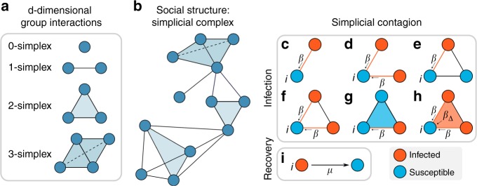
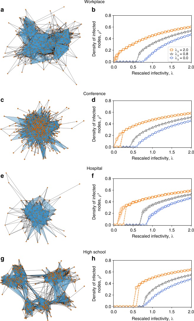
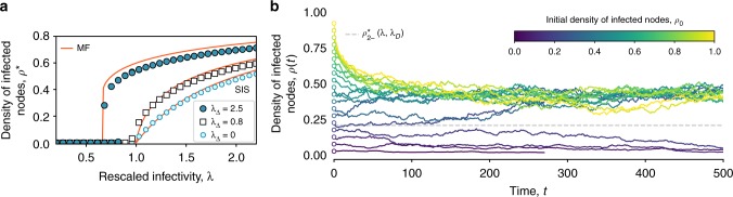
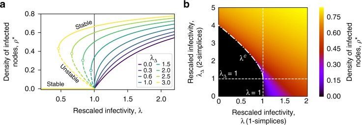
Complex networks have been successfully used to describe the spread of diseases in populations of interacting individuals. Conversely, pairwise interactions are often not enough to characterize social contagion processes such as opinion formation or the adoption of novelties, where complex mechanisms of influence and reinforcement are at work. Here we introduce a higher-order model of social contagion in which a social system is represented by a simplicial complex and contagion can occur through interactions in groups of different sizes. Numerical simulations of the model on both empirical and synthetic simplicial complexes highlight the emergence of novel phenomena such as a discontinuous transition induced by higher-order interactions. We show analytically that the transition is discontinuous and that a bistable region appears where healthy and endemic states co-exist. Our results help explain why critical masses are required to initiate social changes and contribute to the understanding of higher-order interactions in complex systems.

Fig. 1

Simplicial contagion model (SCM). The underlying structure of a social system is made of simplices, representing d-dimensional group interactions (a), organized in a simplicial complex (b). c–h Different channels of infection for a susceptible node i in the simplicial contagion model (SCM) of order D = 2. Susceptible and infected nodes are colored in blue and red, respectively. Node i is in contact with one (c, e) or more (d, f) infected nodes through links (1-simplices), and it becomes infected with probability β at each timestep through each of these links. g, h Node i belongs to a 2-simplex (triangle). In g one of the nodes of the 2-simplex is not infected, so i can only receive the infection from the (red) link, with probability β. In h the two other nodes of the 2-simplex are infected, so i can get the infection from each of the two 1-faces (links) of the simplex with probability β, and also from the 2-face with probability β₂ = β_Δ. i Infected nodes recover with probability μ at each timestep, as in the standard SIS model

Fig. 2

SCM of order D = 2 on real-world higher-order social structures. Simplicial complexes are constructed from high-resolution face-to-face contact data recorded in four different context: a a workplace, c a conference, e a hospital and g a high school. Prevalence curves are respectively reported in panels b, d, f and h, in which the average fraction of infectious nodes obtained in the numerical simulations is plotted against the rescaled infectivity λ = β〈k〉/μ for different values of the rescaled parameter λ_Δ = β_Δ〈k_Δ〉/μ, namely λ_Δ = 0.8 (black triangles) and λ_Δ = 2 (orange squares). The blue circles denote the simulated curve for the equivalent standard SIS model (λ_Δ = 0), which does not consider higher-order effects. For λ_Δ = 2 a bistable region appears, where healthy and endemic states co-exist

Fig. 3

SCM of order D = 2 on a synthetic random simplicial complex (RSC). The RSC is generated with the procedure described in this manuscript, with parameters N = 2000, p₁ and p_Δ tuned in order to produce a simplicial complex with 〈k〉 ∼ 20 and 〈k_Δ〉 ∼ 6. a The average fraction of infected obtained by means of numerical simulations is plotted against the rescaled infectivity λ = β〈k〉/μ for λ_Δ = 0.8 (white squares) and λ_Δ = 2.5 (filled blue circles). The light blue circles give the numerical results for the standard SIS model (λ_Δ = 0) that does not consider higher-order effects. The red lines correspond to the analytical mean field solution described by Eq. (3). For λ_Δ = 2.5 we observe a discontinuous transition with the formation of a bistable region where healthy and endemic states co-exist. b Effect of the initial density of infected nodes, shown by the temporal evolution of the densities of infectious nodes (a single realization is shown for each value of the initial density). The infectivity parameters are set within the range in which we observe a bistable region (λ = β〈k〉/μ = 0.75, λ_Δ = β_Δ〈k_Δ〉/μ = 2.5). Different curves—and different colors—correspond to different values for the initial density of infectious nodes ρ₀ ≡ ρ(0). The dashed horizontal line corresponds to the unstable branch ${\rho }_{2-}^{*}$ of the mean field solution given by Eq. 4, which separates the two basins of attraction

Fig. 4

Phase diagram of the SCM of order D = 2 in mean field approximation. a The stationary solutions ρ* given by Eq. (4) are plotted as a function of the rescaled link infectivity λ = β〈k〉/μ. Different curves correspond to different values of the triangle infectivity λ_Δ = β_Δ〈k_Δ〉/μ. Continuous and dashed lines correspond to stable and unstable branches respectively, while the vertical line denotes the epidemic threshold λ^c = 1 in the standard SIS model that does not consider higher-order effects. For λ_Δ ≤ 1 the higher-order interactions only contribute to an increase in the density of infected individuals in the endemic state, while they leave the threshold unchanged. Conversely, when λ_Δ > 1 we observe a shift of the epidemic threshold, and a change in the type of transition, which becomes discontinuous. b Heatmap of the stationary solution ρ* given by Eq. (4) as a function of the rescaled infectivities λ = β〈k〉/μ and λ_Δ = β_Δ〈k_Δ〉/μ. The black area corresponds to the values of (λ, λ_Δ) such that the only stable solution is ${\rho }_1^{*}=0$. The dashed vertical line corresponds to λ = 1, the epidemic threshold of the standard SIS model without higher-order effects. The dash-dotted line represents the points (λ^c, λ_Δ), with ${\lambda }^c=2\sqrt{{\lambda }_{\Delta }}-{\lambda }_{\Delta }$, where the system undergoes a discontinuous transition

References

1. Albert R, Barabási A-L. Statistical mechanics of complex networks. Rev. Mod. Phys. 2002;74:47. doi: 10.1103/RevModPhys.74.47. - DOI
1. Latora, V., Nicosia, V. & Russo, G. Complex Networks: Principles, Methods and Applications (Cambridge University Press, Cambridge, MA, 2017).
1. Radicchi F, Arenas A. Abrupt transition in the structural formation of interconnected networks. Nat. Phys. 2013;9:717. doi: 10.1038/nphys2761. - DOI
1. Porter, M. A. & Gleeson, J. P. Dynamical Systems on Networks: A Tutorial (Springer, New York, NY, 2005).
1. Barrat, A., Barthelemy, M. & Vespignani, A. Dynamical Processes on Complex Networks (Cambridge University Press, Cambridge, MA, 2008).
Publication types