How single neuron properties shape chaotic dynamics and signal transmission in random neural networks

Abstract

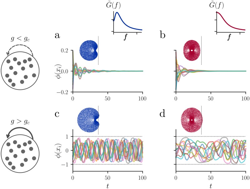
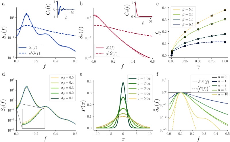
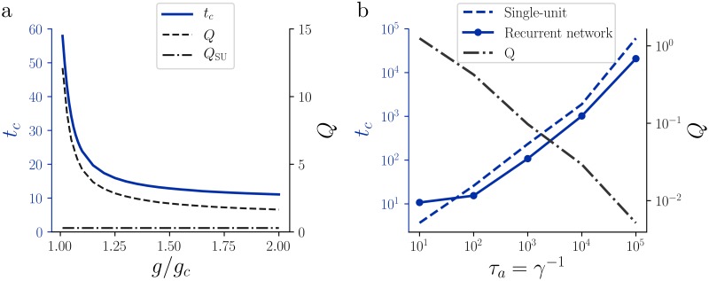
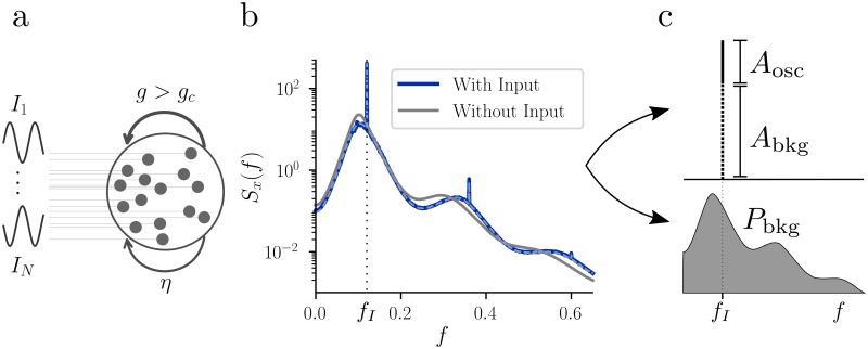
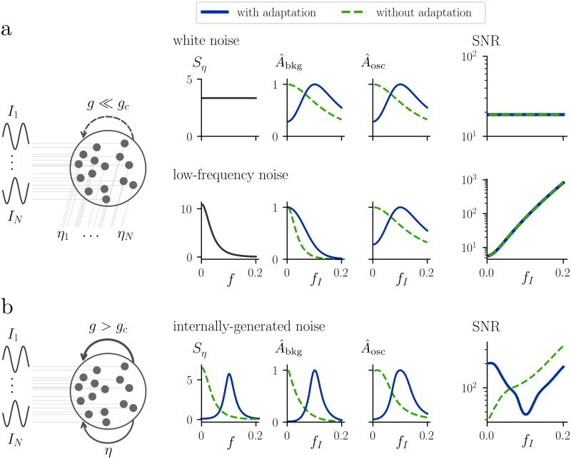
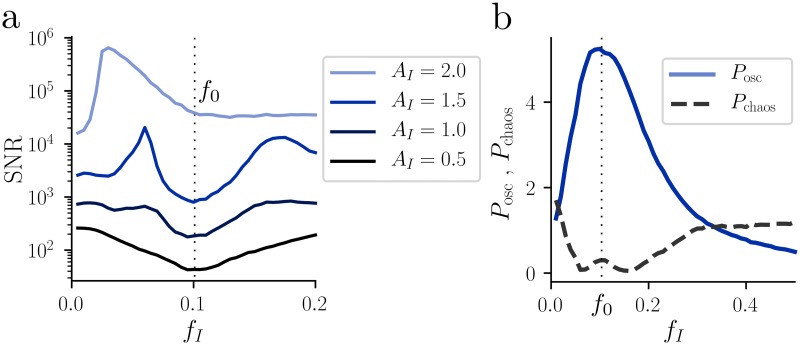
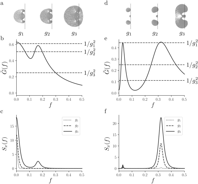
While most models of randomly connected neural networks assume single-neuron models with simple dynamics, neurons in the brain exhibit complex intrinsic dynamics over multiple timescales. We analyze how the dynamical properties of single neurons and recurrent connections interact to shape the effective dynamics in large randomly connected networks. A novel dynamical mean-field theory for strongly connected networks of multi-dimensional rate neurons shows that the power spectrum of the network activity in the chaotic phase emerges from a nonlinear sharpening of the frequency response function of single neurons. For the case of two-dimensional rate neurons with strong adaptation, we find that the network exhibits a state of "resonant chaos", characterized by robust, narrow-band stochastic oscillations. The coherence of stochastic oscillations is maximal at the onset of chaos and their correlation time scales with the adaptation timescale of single units. Surprisingly, the resonance frequency can be predicted from the properties of isolated neurons, even in the presence of heterogeneity in the adaptation parameters. In the presence of these internally-generated chaotic fluctuations, the transmission of weak, low-frequency signals is strongly enhanced by adaptation, whereas signal transmission is not influenced by adaptation in the non-chaotic regime. Our theoretical framework can be applied to other mechanisms at the level of single neurons, such as synaptic filtering, refractoriness or spike synchronization. These results advance our understanding of the interaction between the dynamics of single units and recurrent connectivity, which is a fundamental step toward the description of biologically realistic neural networks.

Fig 1. Microscopic network dynamics with firing rate adaptation.

In the top row (panels a and b), the network is below the bifurcation, (g = 0.96g_c(γ, β)), and it exhibits a transient activity to the stable fixed point. In the bottom row (panels c and d), the fixed point is unstable (g = 1.3g_c) and the network exhibits irregular, self-sustained oscillations. In the left column (panels a and c), the network is in the resonant regime (γ = 0.2, β = 0.5), as it can be seen from the single-neuron linear frequency response function $\tilde{G}\left(f\right)$ (cf. Eq 9). In the right column (panels b and d), the network is in the non-resonant regime (γ = 1, β = 0.1). For each panel, ten randomly chosen units are shown, out of N = 1000 units. Panel c corresponds to the resonant chaotic state, while in panel d the system exhibits chaotic activity similar to the case described in [1]. The insets show the eigenvalue spectrum in the complex plane for the four different sets of parameters. The dashed black line indicates the imaginary axis. Comparing the eigenvalue spectrum of panel a with the one of panel c, we see that the network undergoes a Hopf bifurcation.

Fig 2. Self-consistent statistics in the chaotic regime.

a: Resonant (narrow-band) chaos. Power spectral density obtained from mean-field theory (solid line) and microscopic simulations (light blue, dashed) for γ = 0.25, β = 1 and g = 2g_c(γ, β). The dashed, dark blue line indicates the square modulus of the linear response function $\tilde{G}\left(f\right)$ for the same adaptation parameters. Inset: Normalized mean-field autocorrelation C_x(τ) for the same parameters, plotted against the time lag in units of τ_x. b: Non-resonant (broad-band) chaotic regime. Curves and inset are the same as in a, but with γ = 1, β = 0.1 and g = 2g_c(γ, β). c: Maximum-power frequency f_p of the recurrent network plotted against γ, for different β. Crosses depict results obtained from microscopic simulations, circles show the semi-analytical prediction based on the iterative method and dashed lines shows the theory based on the single neuron response function. For γ = 0 all curves start at f_p = 0. d: Power spectral density S_x(f) for different levels of heterogeneity of the parameter β (solid lines), compared to the case without heterogeneity (dashed line). All the curves are almost superimposed, except at very low frequencies where small deviations are visible (inset). Parameters: γ = 0.25, $\overline{\beta }=1$, $g=2g_c(\gamma ,\overline{\beta })$. e: Distributions P(x) of the activation x from microscopic simulation (N = 2000, solid lines) and theoretical prediction (dashed lines). The adaptation parameter were γ = 0.25 and β = 1. f: Normalized power spectral density ${\widehat{S}}_x\left(f\right)≔S_x\left(f\right)/{\text{max}}_f{S}_x\left(f\right)$ (solid lines) at different iterations n, for the network with adaptation. For the first iterations, the powers of $\widehat{G}\left(f\right)≔\tilde{G}\left(f\right)/{\text{max}}_f\tilde{G}\left(f\right)$ (dashed lines), provide a good approximations of the power spectrum width. The initial power spectral density is a constant and the network parameters are the same as in panel a.

Fig 3. Correlation time and effect of recurrent connections.

a: Correlation time (blue solid line) and Q-factor (dashed line) as a function of the connectivity strength. The weakest connectivity level plotted is g = 1.01g_c(γ, β). Adaptation parameters: γ = 0.1 and β = 1. The dash-dotted horizontal line indicates the Q-factor of a single unit with the same adaptation parameters, driven by white noise. b: Correlation time (blue) and Q-factor (black, dash-dotted line) as a function of the adaptation timescale τ_a ≔ γ⁻¹. Both the recurrent network (solid line) and the single unit driven by white noise (dashed line) scale with τ_a. β = 1 and g = 1.5g_c(γ, β).

Fig 4. Response of the mean-field network to an oscillatory input.

a: Schematic representation of the random network driven by an external input, with phase randomization. For g > g_c, the chaotic activity can be seen as internally-generated noise. b: Effect of an oscillatory external input on the power spectral density S_x(f). In the example, γ = 0.25, β = 1, g = 2g_c(γ, β), f_I = 0.12, while A_I = 0.5 (blue) and A_I = 0 (gray). Simulations (solid blue) and theory (dashed blue) are superimposed. c: Top: Schematic representation of the separation of the power spectral density into its oscillatory (A_osc) and chaotic (A_bkg) components. Note that these quantities depend on the size of the frequency discretization bin. Bottom: Graphical interpretation of P_bkg, i.e. the total variance of the network activity due to chaotic activity (shaded gray area).

Fig 5. Adaptation shapes the SNR in the chaotic regime.

a: For small g, a recurrent network driven by an oscillatory input and external noise can be analyzed in the linear response theory framework. Top row: response of the network to oscillatory drive and independent white noise to each neuron. Bottom row: response of the network to oscillatory drive and independent low-frequency noise to each neuron. For each row, from left to right, we plot the power spectrum of the input noise, the background component of the power spectrum ${\widehat{A}}_{\text{osc}}$, the oscillatory component of the power spectrum ${\widehat{A}}_{\text{osc}}$, and the SNR as a function of the driving frequency. The hat over the symbols A_bkg and A_osc indicates that, to highlight the network shaping, they are normalized to have the same maximum height (equal to one). Notice that, since both signal and noise are shaped in the same way in the linear response framework, the introduction of adaptation does not affect the SNR. b: For large g, the network is subject to internally generated noise and driven by oscillatory input. We plot the same quantities as in panel a. Notice that, due to the nonlinearity of the network, signal and internally-generated noise are shaped in different ways, with the signal being subject to a broader effective filter. As a consequence, the introduction of adaptation in the nonlinear network shapes the SNR by favoring low frequencies. Parameters of the network with adaptation for all panels: γ = 0.25, β = 1 g = 2g_c(γ, β) and A_I = 0.5.

Fig 6. Effect of a strong oscillatory input.

a: SNR at the driving frequency f_I as a function of the driving frequency, for different values of the signal amplitude A_I. As A_I increases, nonlinear interaction between signal and noise become stronger, leading to a qualitative change in the SNR profile. b: Total power of the chaotic (black dashed) and oscillatory (light blue) components of the power spectrum, in the case of strong input (A_I = 1.5). For both panels, γ = 0.25, β = 1.0, and g = 2g_c(γ, β).

Fig 7. Stability of the fixed point and local properties.

a: Critical value of the coupling g_c (color code, right) for different adaptation parameters γ (horizontal axis) and β (vertical axis). The curve β_H(γ) (solid black line) separates the regions of the γ − β plane in which for increasing g we encounter a Hopf bifurcation (above β_H(γ)) or a saddle-node bifurcation (below β_H(γ)). Cross and filled circle: parameters used in Fig 1. Left inset: dependence of g_c on β for fixed γ = 0.9. Top inset: dependence of g_c on γ for fixed β = β_H(γ = 0.9). Blue line: Hopf bifurcation; red line: saddle-node bifurcation. b: Resonance frequency f_m for different adaptation parameters γ, β. Notice that in the non-resonant region the resonance frequency is not defined. Left inset: square-root increase of f_m as a function of β for fixed γ = 0.9. Top inset: non-monotonic behavior of f_m as a function of γ, for fixed β = β_H(γ = 0.9).

Fig 8. Two examples of multi-dimensional rate models.

Parameters defining both models can be found in Table 1. a-b-c: Analysis of a three-dimensional rate model. Eigenvalue spectra (a) corresponding to the coupling values g₁ = 1.28, g₂ = 1.4 and g₃ = 2. The dashed line indicates the imaginary axis. In b we plot the linear response function of the single unit $\tilde{G}\left(f\right)$ (solid line), and the instability threshold corresponding to the three coupling values g₁, g₂ and g₃ (dashed lines). In c we plot the solution of the mean field theory obtained with the iterative method for the three values of g, g₁ = 1.5, g₂ = 2 and g₃ = 3. d-e-f: Same as a,b,c, but for a four-dimensional rate model.

References

1. Sompolinsky H, Crisanti A, Sommers HJ. Chaos in Random Neural Networks. Physical Review Letters. 1988;61(3):259–262. 10.1103/PhysRevLett.61.259 - DOI - PubMed
1. Kadmon J, Sompolinsky H. Transition to Chaos in Random Neuronal Networks. Phys Rev X. 2015;5:041030.
1. van Vreeswijk C, Sompolinsky H. Chaos in neuronal networks with balanced excitatory and inhibitory activity. Science. 1996;274:1724 10.1126/science.274.5293.1724 - DOI - PubMed
1. Rajan K, Abbott LF, Sompolinsky H. Stimulus-dependent suppression of chaos in recurrent neural networks. Phys Rev E. 2010;82:011903 10.1103/PhysRevE.82.011903 - DOI - PMC - PubMed
1. Huang C, Doiron B. Once upon a (slow) time in the land of recurrent neuronal networks…. Current Opinion in Neurobiology. 2017;46:31–38. 10.1016/j.conb.2017.07.003 - DOI - PubMed
Publication types
LinkOut - more resources