Dynamic Causal Modelling of Active Vision

Abstract

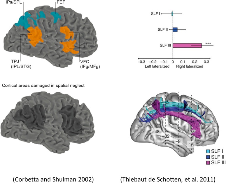
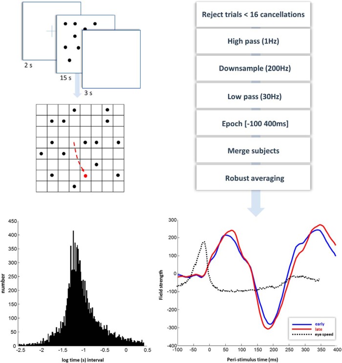
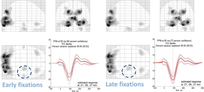
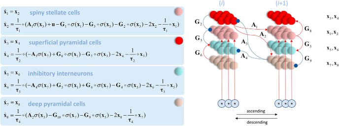
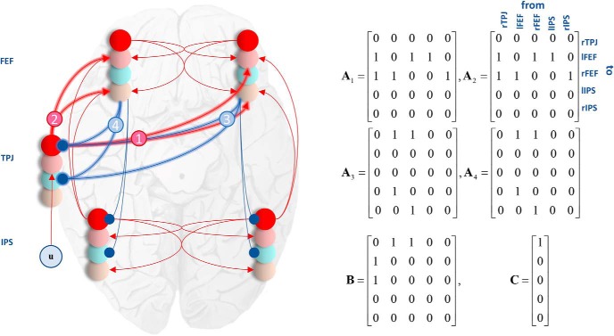
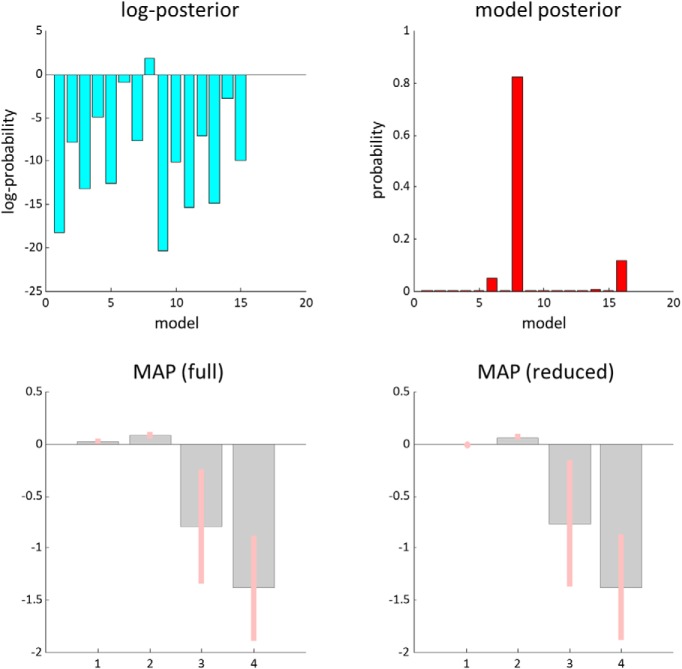
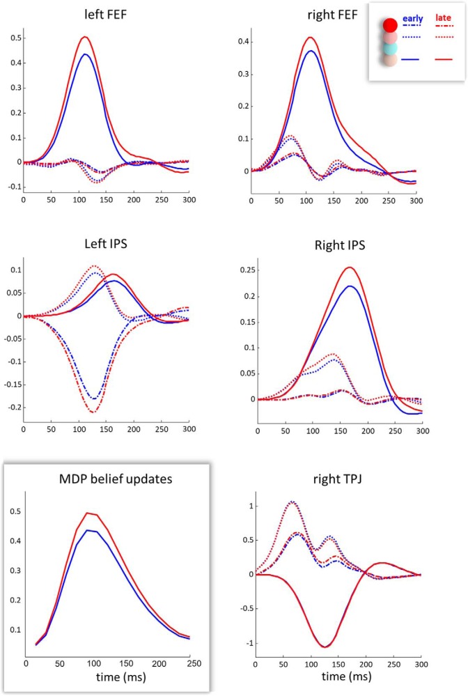
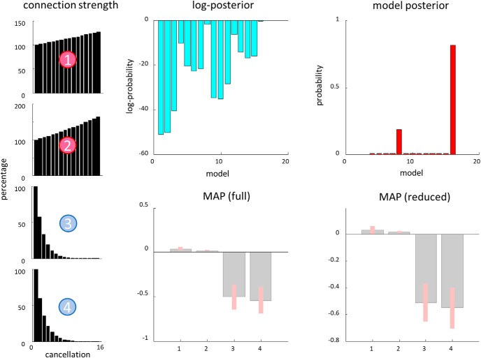
In this paper, we draw from recent theoretical work on active perception, which suggests that the brain makes use of an internal (i.e., generative) model to make inferences about the causes of sensations. This view treats visual sensations as consequent on action (i.e., saccades) and implies that visual percepts must be actively constructed via a sequence of eye movements. Oculomotor control calls on a distributed set of brain sources that includes the dorsal and ventral frontoparietal (attention) networks. We argue that connections from the frontal eye fields to ventral parietal sources represent the mapping from "where", fixation location to information derived from "what" representations in the ventral visual stream. During scene construction, this mapping must be learned, putatively through changes in the effective connectivity of these synapses. Here, we test the hypothesis that the coupling between the dorsal frontal cortex and the right temporoparietal cortex is modulated during saccadic interrogation of a simple visual scene. Using dynamic causal modeling for magnetoencephalography with (male and female) human participants, we assess the evidence for changes in effective connectivity by comparing models that allow for this modulation with models that do not. We find strong evidence for modulation of connections between the two attention networks; namely, a disinhibition of the ventral network by its dorsal counterpart.SIGNIFICANCE STATEMENT This work draws from recent theoretical accounts of active vision and provides empirical evidence for changes in synaptic efficacy consistent with these computational models. In brief, we used magnetoencephalography in combination with eye-tracking to assess the neural correlates of a form of short-term memory during a dot cancellation task. Using dynamic causal modeling to quantify changes in effective connectivity, we found evidence that the coupling between the dorsal and ventral attention networks changed during the saccadic interrogation of a simple visual scene. Intuitively, this is consistent with the idea that these neuronal connections may encode beliefs about "what I would see if I looked there", and that this mapping is optimized as new data are obtained with each fixation.

Keywords: active vision; attention; dynamic causal modelling; eye-tracking; magnetoencephalography; visual neglect.

Figure 1.

The anatomy of attention. Summary of the functional, neuropsychological, and structural characterizations of attention networks in the brain. Top, Left, The components of the dorsal and ventral frontoparietal attention networks, as derived through functional imaging studies. The dorsal sources (blue) are bilaterally activated during visual attention tasks, whereas the ventral (orange) network is lateralized to the right hemisphere. Bottom, Left, Summarizes lesion studies that demonstrate that lesions to the ventral network in the right hemisphere are associated with visual neglect. Bottom, Right, The three branches of the superior longitudinal fasciculus; a white-matter tract that connects the sources of the attention networks. The plot on the top right indexes the lateralization of these tracts by their relative volumes in each hemisphere. Notably, the third branch, which connects the ventral sources, is significantly right lateralized. Left images are reprinted by permission from Springer Nature: Nature Reviews Neuroscience from (Corbetta and Shulman, 2002), and those on the right reprinted by permission from Springer Nature: Nature Neuroscience from (Thiebaut de Schotten et al., 2011). The material in this figure is not included in the CC BY license for this article. STG, Superior Temporal Gyrus; VFC, Ventral Frontal Cortex; SPL, Superior Parietal Lobule. ***p < 0.001.

Figure 2.

Oculomotor cancellation task and preprocessing. Top, Left, The sequence of events for a given trial. First, a fixation cross is presented for 2 s. After this, a display with 16 black dots is randomly generated and presented for 15 s. This is followed by a blank screen for 3 s. The dots were placed within an 8 × 8 grid (not visible to the participants), as shown at the bottom. When the dots were visible on screen, we tracked the eyes of the participant. Whenever their gaze entered a square containing a black dot, this changed from black to red and remained red for the rest of the trial. Participants were instructed to look at the black dots, and to avoid looking at red dots. Events were defined as the time at which the eye crossed into the square, causing a change in color (i.e., a cancellation). There were 15 of these trials per block, with 6 blocks per participant. The bottom left plot shows a histogram of the time intervals between saccadic dot cancellations, to give a sense of the latency between saccades. These latencies are reported using a (natural) logarithmic time scale (with time in seconds) over the first 2.5 SD above and below the mean. The mean here is −1.0597, corresponding to ∼3 cancellations per second (consistent with the 3–4 Hz frequency of saccadic sampling; Hoffman et al., 2013). Right, The sequence of preprocessing steps used and the first principal component of the ensuing evoked response. The evoked response to early cancellations is averaged from 6738 events, and the response to late cancellations from 6571. Superimposed upon this is a trace of the eye speed in peristimulus time in arbitrary units. This is aligned so that zero corresponds to the average speed during the time in which the fixation cross was present.

Figure 3.

Source reconstruction with multiple sparse priors. These images show the Bayes optimal source reconstruction under multiple sparse priors (and following application of a temporal Hanning window) for the first eight cancellations (left) and the second eight cancellations (right) in a trial. This reveals a set of symmetrical sources in both the frontal and posterior cortical sources, with a right lateralized temporal component. The striking asymmetry of these temporal sources (dashed circles) is encouraging, considering the known rightward lateralization of the ventral attention network. Although we might expect the frontal sources to be more dorsal, this may reflect the ill-posed nature of MEG source localization; there are many possible combinations of sources in 3D space that could give rise to the same pattern of activation over the 2D sensory array. The estimated responses show the greatest amplitude at ∼100 ms. In the left plot (showing the maximal response for the first condition), the red lines indicate the reconstructed activity from the early cancellations and gray from the late cancellations. In the right plot (maximal response for the second condition), red is late and gray is early. Bayesian credible intervals are shown as dotted lines for each response. The confidence associated with the posterior probability maps (PPM; Friston and Penny, 2003), in addition to the variance explained, are included in the top left of each plot, and the location at which the response is estimated is given at the bottom right.

Figure 4.

The canonical microcircuit. The equations on the left of this schematic describe the dynamics of the generative model that underwrites the dynamic causal modeling in this paper. The x vectors represent population-specific voltage (odd subscripts) and conductance (even subscripts). Each element of the x vectors represents a distinct cortical source. The notation a ○ b means the element-wise product of a and b. The matrix A determines extrinsic (between-source) connectivity (here illustrated as connections between a lower source i and a higher source i+1), whereas G determines the intrinsic (within-source) connectivity. Subscripts for these matrices indicate mappings between specific cell populations. For example, A₁ describes ascending connections from superficial pyramidal cells (source i) to spiny stellate cells (source i+1), whereas A₃ describes descending connections from deep pyramidal cells (source i+1) to superficial pyramidal cells (source i). Experimental inputs, in our case, the cancellation of the target on fixation, are specified by u. Right, The neuronal message passing implied by these equations. Red arrows indicate excitatory connections and blue inhibitory. Superficial pyramidal cells give rise to ascending connections that target spiny stellate and deep pyramidal cells in a higher cortical source. Descending connections arise from deep pyramidal cells that target superficial pyramidal cells and inhibitory interneurons.

Figure 5.

Network architecture. This schematic illustrates the form of the network model we used to test our hypothesis. The dorsal network is present bilaterally (FEF and IPS) and is connected to the ventral network, represented by the TPJ, on the right. The TPJ receives input as it sits lower in the visual hierarchy than the FEF (Felleman and Van Essen, 1991). Our hypothesis concerns the (highlighted) connections between the two networks. We compared models that allowed for changes or visual search-dependent plasticity in connections from the TPJ to left FEF (1), from the TPJ to right FEF (2), from the left FEF to TPJ (3), from the right FEF to TPJ (4), and every combination of the above. The matrices on the right illustrate the specification of these connections. The A matrices are the same as those in Figure 4 and represent extrinsic connections between sources (with subscripts indicating which specific cell populations in those sources). B specifies the connections that can change between the early and late cancellations and C specifies which sources receive visual (i.e., geniculate) input. To ensure that the signs of the A (and C) connections do not change during estimation, their logarithms are treated as normally distributed random variables. This ensures an excitatory connection cannot become an inhibitory connection and vice versa.

Figure 6.

Model comparison and Bayesian model averaging. This figure shows the results of comparing models with different combinations of condition-specific effects on the forward and backward connections between the right TPJ and the FEFs. We performed this comparison using Bayesian model reduction (Friston et al., 2017), which involves fitting a full model that allows all four connections to change and analytically evaluating the evidence for models with combinations of these changes switched off. The top plots show the log posterior probabilities associated with each model, and the posterior probabilities. The winning model (number 8) allows for modulation in Connections 2, 3, and 4 (Fig. 5). The bottom plots show that, for the later fixations, there is a modest increase in the effective connectivity in Connection 2, but a decrease in 3 and 4. These values correspond to log scaling parameters, such that a value of zero means no change. The bottom left plot shows these parameter (maximum a posteriori) estimates for the full model (that allows for all connections). The bottom right plot shows the Bayesian model average of these estimates (weighted by the probability of each reduced model to account for uncertainty over models). Bayesian 90% credible intervals are shown as pink bars.

Figure 7.

Estimated neuronal activity. These plots show the estimated activity in each excitatory cell population. Dashed lines indicate the superficial pyramidal cells that give rise to ascending connections and are inhibited by higher cortical sources. Ascending connections target the spiny stellate cells (dotted lines), and the deep pyramidal cells (unbroken lines). The latter give rise to descending connections. The activity here is shown for early (blue) and late (red) cancellations, for each of the cortical areas shown in Figure 5. The bottom left plot (highlighted) shows the simulated evoked responses obtained from the Markov decision-process model described by Parr and Friston (2017b), drawing from the process theory associated with active inference (Friston et al., 2016). It is computed by taking the absolute rate of change of the sufficient statistics of posterior beliefs about the current fixation location, summed over spatial scales (please see the discussion for details). Whereas the y-axis here is arbitrary, the x-axis extends to 250 ms, consistent with the theta frequency of saccadic eye movements. There is a striking resemblance between the simulated rate of belief updating and the FEF neuronal activity estimated from our empirical data.

Figure 8.

Time-dependency of modulatory changes. The plots on the right are the same as those in Figure 6, but modeling a parametric effect of number of previous cancellations. For this model, in place of the early and late conditions, we treated each sequential cancellation as a separate event. Because the model is parameterized in terms of log-scaling parameters, linear (i.e., [0,1,…,15]) parametric effects of time (number of previous cancellations) correspond to a monoexponential change in coupling [starting from a strength of exp(0), corresponding to 100%]. The two most probable models are the same as in Figure 6, and the overall pattern of changes shown in the MAP estimates is the same (but with some evidence in favor of a small change in Connection 1). The plots on the left show the estimated changes in each connection with successive cancellation events, as a percentage of their initial values. These indicate an increase in the strength of forward excitatory connections over time, and a decrease in backward inhibitory connections.

References

1. Albert ML. (1973) A simple test of visual neglect. Neurology 23:658–664. 10.1212/WNL.23.6.658 - DOI - PubMed
1. Andreopoulos A, Tsotsos J (2013) A computational learning theory of active object recognition under uncertainty. Int J Comput Vis 101:95–142. 10.1007/s11263-012-0551-6 - DOI
1. Antonini M, Barlaud M, Mathieu P, Daubechies I (1992) Image coding using wavelet transform. IEEE Trans Image Process 1:205–220. 10.1109/83.136597 - DOI - PubMed
1. Barlow HB. (1961) Possible principles underlying the transformations of sensory messages. In: Sensory communication (Rosenblith W, ed), pp 217–234. Cambridge, MA: MIT.
1. Barlow HB. (1974) Inductive inference, coding, perception, and language. Perception 3:123–134. 10.1068/p030123 - DOI - PubMed
Publication types
MeSH terms
LinkOut - more resources