qPCR data analysis: Better results through iconoclasm

Abstract

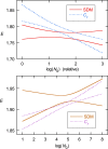
The standard approach for quantitative estimation of genetic materials with qPCR is calibration with known concentrations for the target substance, in which estimates of the quantification cycle (C_q ) are fitted to a straight-line function of log(N ₀), where N ₀ is the initial number of target molecules. The location of C_q for the unknown on this line then yields its N ₀. The most widely used definition for C_q is an absolute threshold that falls in the early growth cycles. This usage is flawed as commonly implemented: threshold set very close to the baseline level, which is estimated separately, from designated "baseline cycles." The absolute threshold is especially poor for dealing with the scale variability often observed for growth profiles. Scale-independent markers, like the first derivative maximum (FDM) and a relative threshold (C_r ) avoid this problem. We describe improved methods for estimating these and other C_q markers and their standard errors, from a nonlinear algorithm that fits growth profiles to a 4-parameter log-logistic function plus a baseline function. Further, by examining six multidilution, multireplicate qPCR data sets, we find that nonlinear expressions are often preferred statistically for the dependence of C_q on log(N ₀). This means that the amplification efficiency E depends on N ₀, in violation of another tenet of qPCR analysis. Neglect of calibration nonlinearity leads to biased estimates of the unknown. By logic, E estimates from calibration fitting pertain to the earliest baseline cycles, not the early growth cycles used to estimate E from growth profiles for single reactions. This raises concern about the use of the latter in lengthy extrapolations to estimate N ₀. Finally, we observe that replicate ensemble standard deviations greatly exceed predictions, implying that much better results can be achieved from qPCR through better experimental procedures, which likely include reducing pipette volume uncertainty.

Keywords: Calibration; Chi-square; Cq, quantification cycle; Ct, threshold cycle, where y = yq; Cy0, intersection of a straight line tangent to the curve at the FDM with the baseline-corrected x-axis; Data analysis; E, amplification efficiency; FDM and SDM, cycles where y reaches its maximal first and second derivatives, respectively; LS, least squares; N0, initial number of target molecules in sample; S, sum of weighted, squared residuals (= "Chisq" in KaleidaGraph fit results, = Χ2 when wi = 1/σi2); SD, standard deviation; SE, parameter standard error; Statistical errors; Weighted least squares; qPCR; qPCR, quantitative polymerase chain reaction; wi, statistical weight for ith data point; y and y0, fluorescence signal above baseline at cycle x and at cycle 0; yq, signal at x = Cq; Χ2, chi-square; ν, statistical degrees of freedom, = # of data points - # of adjustable parameters; σ2a and σ, variance and standard deviation.

Fig. 1

qPCR fluorescence curves for lambda gDNA for 10-fold dilution from 188,000 copy numbers to 19, as recorded in triplicate by Rutledge and Stewart [7]. Inset shows positions of C_q markers for one reaction at highest concentration. With the threshold set at 12% of the (plateau – baseline) difference, the relative threshold C_r coincides with Cy0 within 0.1 cycle.

Fig. 2

Results of LS fits of 4 C_q markers from growth profiles in Fig. 1 to linear relation (right) and of FDM to quadratic centered at log(N₀) = 3 (top). The quadratic coefficient in the latter is statistically significant in ad hoc fitting, having magnitude larger that its SE. Note close agreement in slopes (giving E) and in "Chisq" values (sums of squared residuals) for linear fits. C_q values were obtained from log-logistic fits of 24-point regions of profiles centered near the half-intensity points.

Fig. 3

NLS fits of first reaction at highest concentration in 94 × 4 Reps dataset [10] to LL4 + bas(x) = a + bx + cx², in normal (upper) and alternate (alt) modes. The quantity D in the denominator of LL4 is as defined in Eq (11). Chisq is the sum of squared residuals for these unweighted fits.

Fig. 4

Standard deviations/errors for each of 4 concentrations in the 94 × 4 Reps data [10]. Ensemble SDs at top from present estimates of Cy0, compared with best from [10] and C_r,x estimates from [15]. At bottom are the rms (root-mean-square) averages of the parametric SEs from the individual fits, for Cy0 using LL4 model in alt mode, and for C_r,_x. Connecting lines are just for display purposes.

Fig. 5

Ensemble variances for absolute and relative threshold in the 94 × 4 Reps data. For C_t, y_q = 700; for C_r,x, r = 0.18. Estimates for both were obtained by fitting to Eq. (2) plus the bas(x) function of Eq. (15). Error bars represent one SD. The average C_t values slightly exceed those for C_r,x, by from 0.07 to 0.30.

Fig. 6

Calibration fits of C_q estimates for 94 × 4 Reps data, weighted using a common set of inverse ensemble variances. At top are linear, quadratic, and cubic fits of the C_r estimates to polynomials in (x –1.5), showing that the cubic coefficient (d) is not statistically defined but that the quadratic one (c) is. For comparison, the quadratic fits of Cy0, FDM, and SDM are included, confirming that c is statistically significant in every case and showing that all E estimates are statistically consistent at x = 1.5.

Fig. 7

Amplification efficiency as a function of concentration, from quadratic fit results in Fig. 6. Error bars (1-σ) are shown for just Cy0 but are nearly identical for all 4 markers.

Fig. 8

Estimating data variance from polynomial fitting, for 4th dilution in 3 × 5 data from [7], in plateau (A) and baseline (B) regions. The estimated variances are Chisq/(n–5), with n = 14 in the plateau region and 22 in the baseline region. Fit results are shown for only the lowest curve in each panel; Chisq values for the other curves (open and solid points, respectively) are 27,000 and 14,700 (A) and 1056 and 4080 (B). Note that none of the parameters in A is statistically significant; in fact these data are well represented by a quadratic function, with little increase in Chisq but an increase of 2 in ν, giving ∼20% smaller estimated variances.

Fig. 9

Fit of estimated variances for 3 × 5 data from [7] to Eq. (16). From these results, the second term dominates the variance even in the baseline region.

Fig. 10

C_q variance estimates from replicate values in Table 1, displayed in logarithmic form, and results from fitting values for each marker to ln ($A+{{\sigma }^2}_{C_q,\text{Pois}}$), where the Poisson variance is given by Eq. (8), with E taken as 1.915. Error bars are shown for C_r only but are the same for all, σ = 1. Values of A range from 0.00015 for Cy0 to 0.0011 for SDM.

Fig. 11

C_q variance estimates from Lievens data [32], displayed and fitted as in Fig. 10, with E taken as 1.86 and N₀ = 160 for the lowest concentration. Error bars shown for C_r,x are representative of the others.

Fig. 12

Dependence of AE on N₀ from cubic calibration fits of C_q estimates for data from [32]. Error bars shown for FDM are comparable for all. χ² in the calibration fits ranged from 87 for Cy0 to 112 for SDM (90 C_q values).

Fig. 13

1-σ confidence bands for extreme estimates of E as functions of log(N₀) for data from [23] (lower) and [33] (upper). For the former (84 reactions), χ² values for FDM, SDM, C_r, Cy0, and C_r,x were, respectively, 100, 500, 109, 183, and 109; in the same order the χ² values for the latter (72 reactions) were 80, 79, 62, 66, and 71.

Fig. 14

rms parametric SE values for the different C_q markers, averaged over all concentrations in each dataset. These SEs generally vary little with concentration.

Fig. 15

χ² values from the weighted calibration fits for the different C_q markers, normalized to unity for each dataset. In each case, common weights were used for the 5 C_qs.

References

-
- Tellinghuisen J. Using nonlinear least squares to assess relative expression and its uncertainty in real-time qPCR studies. Anal. Biochem. 2016;496:1–3. - PubMed
- Bustin S.A. Absolute quantification of mRNA using real-time reverse transcription polymerase chain reaction assays. J. Mol. Endocrinol. 2000;25:169–193. - PubMed
LinkOut - more resources
Full Text Sources
Research Materials