Metabolic network percolation quantifies biosynthetic capabilities across the human oral microbiome

Abstract

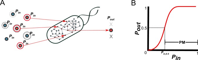
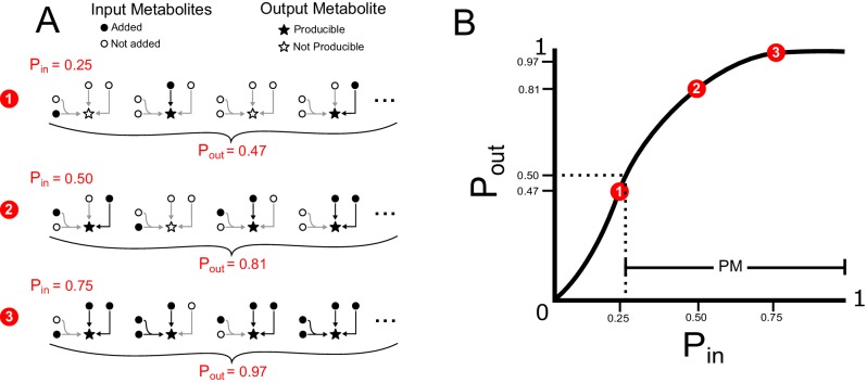
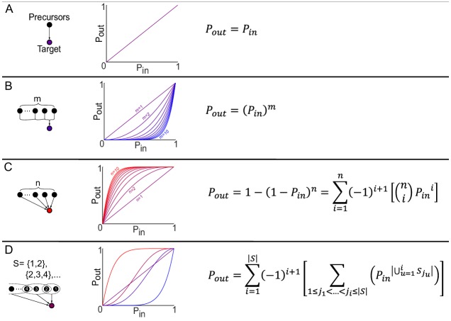
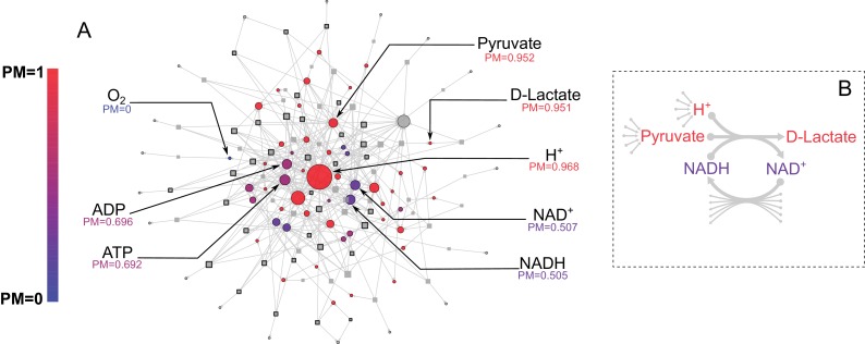
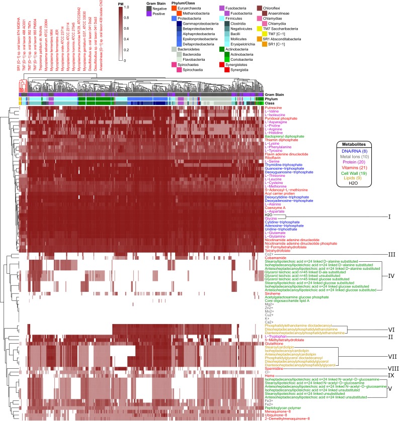
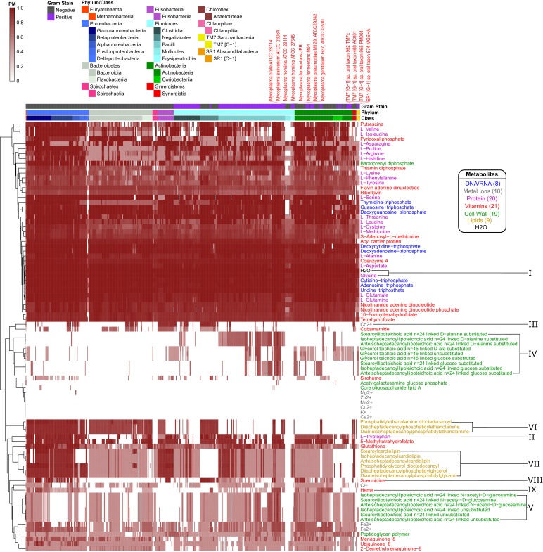
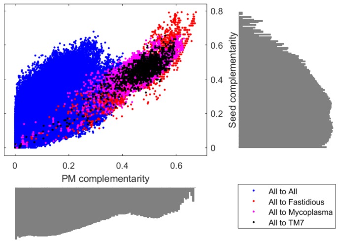
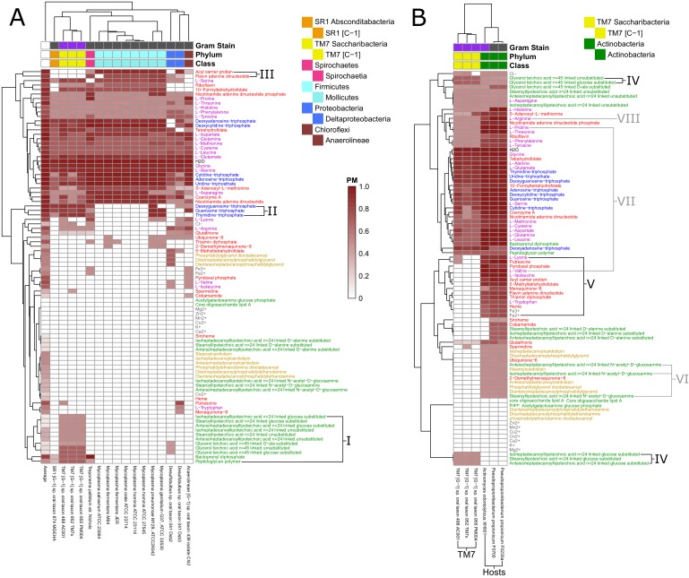
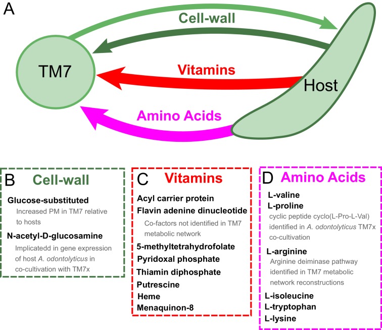
The biosynthetic capabilities of microbes underlie their growth and interactions, playing a prominent role in microbial community structure. For large, diverse microbial communities, prediction of these capabilities is limited by uncertainty about metabolic functions and environmental conditions. To address this challenge, we propose a probabilistic method, inspired by percolation theory, to computationally quantify how robustly a genome-derived metabolic network produces a given set of metabolites under an ensemble of variable environments. We used this method to compile an atlas of predicted biosynthetic capabilities for 97 metabolites across 456 human oral microbes. This atlas captures taxonomically-related trends in biomass composition, and makes it possible to estimate inter-microbial metabolic distances that correlate with microbial co-occurrences. We also found a distinct cluster of fastidious/uncultivated taxa, including several Saccharibacteria (TM7) species, characterized by their abundant metabolic deficiencies. By embracing uncertainty, our approach can be broadly applied to understanding metabolic interactions in complex microbial ecosystems.

Keywords: Saccharibacteria (TM7); computational biology; human microbiome; metabolic modeling; oral microbial flora; oral prokaryotes; systems biology; uncultivated bacteria.

Figure 1.. A probabilistic framework for calculating the producibility metric (PM).

(A) Random samples of input metabolites are added to the metabolic network with probability P_in. Samples are shown here with gray or red circles. Sampled input metabolites are then used to calculate if a specified target output metabolite can be produced or not. Here the solid red circled sample leads to production of the target metabolite while the dotted gray circled samples do not. The probability of producing the target output metabolite (P_out) is calculated by taking many random samples at a specified P_in. (B) A producibility curve is calculated which represents P_out as function of P_in. Points along this curve are sampled by assigning the P_in value and estimating P_out. The P_in value at which P_out = 0.5 (P_in,0.5) is used to define the producibility metric (PM) as PM = 1-P_in,0.5.

Figure 1—figure supplement 1.. Probabilistic framework simple example.

(A) Input probabilities (P_in) are assigned to each input metabolite to designate the probability of adding that metabolite to the network. Random sets of input metabolites are sampled, based on P_in, and a modified version of flux balance analysis is used to determine if the network can produce a specified target output metabolite for each random sample. Many random samples are taken to estimate the output probability (P_out) of the target output metabolite. Three examples of P_in values and the corresponding P_out values are shown for a very simple network with three reactions, four input metabolites and one target metabolite. For this simple example, the output probabilities can be calculated using the probabilistic equation ${\displaystyle P_{out}=1-\left[{\left(1-P_{in}\right)}^2\ast \left(1-P_{in}^2\right)\right]=2P_{in}-2P_{in}^3+P_{in}^4}$. For more information on this theoretical calculation please refer to Figure 1—figure supplement 2. (B) A producibility curve is calculated which represents P_out as a function of P_in. Points along this curve are sampled by assigning the P_in value and estimating P_out. The three examples from A are shown in red on the curve in B. The PM is equal to one minus the value of P_in at which P_out equals 0.5 (P_in,0.5), such that increasing PM correspond to increasing producibility. In our implementation the PM for a particular metabolic network and metabolite is calculated efficiently using a non-linear fitting algorithm to find P_in,0.5. For further details on our exact implementation see the methods section “Algorithm functions: calc_PM_fit_nonlin.

Figure 1—figure supplement 2.. Theoretical properties of the producibility curve.

Theoretically, our method is closely related to the minimal precursor sets of a metabolic network. The minimal precursor sets describe all minimal subsets of metabolites that can be used to synthesize a particular metabolite or set of metabolites. A combinatorial formula was developed to calculate the value of P_out from the set of minimal precursor sets (S) and the value of P_in. Using this formula, an exact producibility curve can be plotted and theoretical values of the producibility metric (PM) can be calculated. This calculation is shown for increasingly complicated and general minimal precursor set structures. (A) In the simplest case, a single metabolite serves as the minimal precursor set for the target. This leads to a straight line producibility curve (P_out = P_in) and an expected PM value of 0.5. (B) If the target metabolite can be produced from one minimal precursor set of size m P_out is equal to P_in raised to the power of m due to the assumption that all metabolites are added independently. As m increases the producibility curve bows outward towards P_in = 1, and the PM decreases below 0.5. (C) If the target metabolite can be produced from n different minimal precursor sets of size 1 P_out can be defined based on the probabilistic rule for an or relationship, or it can be represented with a combinatorial formula. $\left(\begin{array}{c}n\\ i\end{array}\right)$ represents the binomial coefficients for n choose i. As n increases the producibility curve bows inward towards P_in = 0, and the PM increases above 0.5. (D) In the most general case, minimal precursor sets can be overlapping and any size/number. The producibility curve and PM vary depending on these properties. A combinatorial formula can be used to represent this general case. $\left|S\right|$ is the cardinality of the set of minimal precursor sets (the total number of minimal precursor sets). $\left|{\bigcup }_{u=1}^i{S}_{j_u}\right|$ is the cardinality of the union of the minimal precursor sets being enumerated by the recursive sum (the number of unique metabolites in the combination of minimal precursor sets being enumerated). The recursive sum over j_i enumerates all possible combinations of i minimal precursor sets by summing over the indices j_i where j_i is between j_i-1 and $\left|S\right|$, thus enumerating binomial combinations. The outer sum implements the inclusion exclusion principle.

Figure 2.. E. coli core metabolic network metabolite producibility.

(A) The E. coli core metabolic network is represented as a bipartite graph with metabolites shown as circles and reactions shown as squares. Reactions shown with a black border are irreversible in the model, those with no border are reversible. All intracellular metabolites are colored based on their PM value (low – blue, high – red). Reactions and metabolite nodes are sized based on their total node degree. Several key metabolites of interest are highlighted with their corresponding PM values shown. Central metabolites such as H⁺ and Pyruvate have high degree and high PM. Cofactors such as AMP/ADP/ATP and NAD⁺/NADH have high degree but low PM, as they cannot be synthesized in this network. Oxygen is an example of a PM=0 metabolite that cannot be produced from any other metabolites in this network. D-lactate is an example of a metabolite with low degree and high PM that is it is easily produced but not well-connected. (B) The lactate dehydrogenase reaction producing D-Lactate is shown as an example to illustrate that poorly connected metabolites can display a high PM, and how recycled cofactors have minimal impact on PM values. Lactate dehydrogenase produces D-lactate and NAD⁺ from pyruvate, H⁺ and NADH. The metabolite D-lactate has high PM despite being produced only by this one reaction in the metabolic network because it can be produced from the high PM metabolites pyruvate and H⁺, which are themselves produced from a large number of possible precursors. Although NADH is also used to produce D-lactate, and has a relatively low PM in this core model, it has minimal impact on the PM of D-lactate as NADH can be recycled from NAD⁺ by a large number of reactions (represented by the arrows at the bottom of the figure) and thus production of NADH is not necessary for the production of D-lactate.

Figure 2—figure supplement 1.. Node degree and producibility metric do not correlate for E. coli core metabolic network intracellular metabolites.

Different forms of the node degree (ND) are plotted against the producibility metric (PM) for all intracellular metabolites in the E. coli core network. No correlation (Spearman’s rank correlation) is observed between the PM and any form of node degree. (A) The in node degree (ND in) is the sum of the number of reactions producing the metabolite. (B) The out node degree (ND out) is the sum of the number of reactions consuming the metabolite. (C) The total node degree (ND total) is the sum of the in and out node degrees. (D) The total degree without double counting reversible reactions (ND total no Rev) is the total node degree when counting reversible reactions only once.

Figure 2—figure supplement 2.. Producibility analysis of the histidine biosynthetic pathway.

(A) A network representation of the histidine biosynthetic pathway is shown. Reactions are represented as squares, histidine is shown as a red circle, main intermediate metabolites are shown as black circles, cofactors metabolites are shown as gray circles. Different histidine auxotrophs were generated by removing reactions at increasing distance from histidine in the E. coli iJO1366 metabolic network. (B) The producibility metric (PM) for histidine was calculated for the different simulated E. coli auxotrophs (blue dots). The theoretical PM values, calculated using the formula from Figure 1—figure supplement 2C and assuming minimal precursor sets of size corresponding to the number of main intermediate metabolites that remain attached to histidine in a particular auxotroph are also plotted (black X’s). (C) The presence of the histidine biosynthetic pathway was measured across 456 different oral microbiome metabolic networks in two different ways: pathway sum – the total number of reactions from the pathway present in an organism’s metabolic network, and pathway length – the number of reactions in the pathway starting at histidine and counting until the first missing reaction. These two metrics were compared to the PM for histidine across oral microbiome organisms, both metrics were correlated with the PM for histidine with pathway length being more strongly correlated (pathway sum: spearman correlation = 0.79, p-value=8.5e-99; pathway length: spearman correlation = 0.88, p-value=3.6e-145).

Figure 3.. The accuracy of flux balance analysis and the producibility metric for different perturbed E. coli genome-scale metabolic networks.

Reactions were randomly removed from the E. coli iJO1366 metabolic network generating 50 different networks at five different levels of reaction removal. These networks were then analyzed with the producibility metric (PM) and flux balance analysis (FBA) in a minimal and complete medium. The accuracy of the PM and FBA results were assessed through two different measures and plotted as a function of the number of reactions removed on a semi-log plot. (A) Quantitative difference accuracy – The accuracy was measured quantitatively based on the L1 norm of the difference between the original network metric and the randomly perturbed network metric. For FBA the L1 norm was computed as the absolute value of the difference between the biomass flux of the original network and the perturbed network. For the PM the L1 norm was calculated as the sum of the absolute value of the difference between each PM value. The L1 norm for both metrics was then normalized and subtracted from one to give a measure of accuracy. The mean of 50 different randomly perturbed networks at five different reaction removal levels is shown with dots connected by solid lines (FBA on minimal medium: Blue, FBA on complete medium: Red, PM: Purple). The standard error of the metric is shown as a shaded region around the line. (B) Biomass production accuracy – The accuracy was measured by the fraction of randomly perturbed metabolic networks that were capable of producing biomass. For FBA this was calculated as the fraction of networks capable of producing biomass flux above 1% of the unperturbed biomass flux (FBA on minimal medium: Blue, FBA on complete medium: Red). For the PM, the biomass production accuracy was calculated as the fraction of networks capable of producing all biomass components above a specified PM threshold. The threshold was either PM >0.1 (solid purple) or PM >0.6 (dashed purple).

Figure 3—figure supplement 1.. E. coli auxotroph co-cultures metabolite producibility.

(A) The producibility metric (PM) was calculated for all essential biomass metabolites for different E. coli auxotrophs that were co-cultured in Wintermute and Silver (2010). Auxotrophs were simulated from the E. coli iJO1366 metabolic network. The genes removed in the auxotroph are labeled along the rows. The metabolites are labeled along the columns. Auxotroph PM vectors were clustered hierarchical using average distances between clusters. The overall distance between auxotroph PM values was positively correlated with synergistic growth from Wintermute and Silver (2010) (Mantel test: rho = 0.1919, p-value=0.0181). (B) The amino acid PM values are extracted and sorted to demonstrate the reduced PM of amino acids with knock-outs in their pathway. Auxotrophs are shown on the row labels, grouped by the amino acid pathway of the auxotroph. Amino acids are shown on the column labels ordered in corresponding order to the auxotrophs. Trends are highlighted by colored outlines. Green outlines show auxotrophs within the same pathway that show corresponding decrease in PM for the associated amino acid. The blue outline shows a cross-pathway interaction where an auxotroph in the glutamine pathway causes a decrease in histidine PM. The purple outline shows an auxotroph in the branched chain amino acid pathway that has decreased PM for branched chain amino acids, but increased synergistic growth with other auxotrophs of this pathway. (C) Co-culture growth data from Wintermute et al. is plotted for 28 amino acid auxotrophs (average of day 4 replicates 1 and 2 from supplemental information of Wintermute and Silver, 2010). Trends are highlighted by colored outlines. Green outlines demonstrate auxotrophs in the same pathway that result in decreased synergistic growth. The blue outline illustrates an example of a cross-pathway interaction where an auxotroph in the glutamine pathway shows decreased synergistic growth with auxotrophs in the histidine pathway. The purple outline demonstrates an unexpected result where an auxotroph in the branched chain amino acid pathway shows increased synergistic growth with other auxtrophs in branched chain amino acid pathways. (D) The correlation between auxotrophs PM values and average synergistic growth across all partner auxotrophs was calculated. For the entire dataset, there was no significant correlation between average PM and average synergistic growth (Spearman’s ρ: −0.1671, p-value: 0.2662). However, for the specific example of knockouts in the tryptophan biosynthetic pathway, we observed a significant correlation between tryptophan PM and average synergistic growth (Spearman’s ρ: 1.000, p-value: 0.0167).

Figure 4.. Human oral microbiome organisms PM matrix.

The producibility metric (PM) was calculated for 456 different oral microbiome organisms (columns) and 88 different essential biomass metabolites (rows). The resulting matrix is hierarchically clustered based on average distances between organisms and metabolites PM values. Organism Gram-stain and phylum/class are indicated by several annotation columns at the top of the matrix. The biomass metabolites analyzed consisted of several different types of metabolites indicated with different colors. Several metabolites that showed interesting patterns across oral microbiome organisms are highlighted with roman numerals. The most distinct cluster of organisms, highlighted and annotated (top left), consisted of fastidious reduced-genome organisms (Mycoplasma, Treponema) and uncultivated or recently cultivated organisms (SR1, TM7, Desulfobulbus, Anaerolineae).

Figure 4—figure supplement 1.. Taxonomically ordered human oral microbiome organisms PM matrix.

The producibility metric (PM) was calculated for 456 different oral microbiome organisms (columns) and 88 different essential biomass metabolites (rows). The columns are arranged in taxonomic order based on phylum and class, and the rows are clustered hierarchically based on average distances between PM values.

Figure 4—figure supplement 2.. Prediction of average producibility metric using genome size and taxonomic parameters.

(A) The average producibility metric (PM) across all biomass metabolites for each organism is correlated with the log of the genome size (log base 10 of base pairs) for each organism. A linear (blue) and quadratic (red) regression model are shown. (B, C) The fit is improved when adding nominal taxonomic parameters of varying resolution. The Akaike information criterion (AIC), and the Bayesian information criterion (BIC) are plotted to summarize the improvement in model performance as nominal taxonomic parameters are added on top of genome size to the regression model. A linear regression model is shown in blue and quadratic model in red. Improved fit is indicated by a decreased AIC or BIC value. The AIC tends to be biased towards overly complex models while the BIC has a larger penalty for additional parameters that biases it towards simpler models. The AIC improves up to the genus taxonomic level and the BIC improves up to the order level, indicating that the data can be additionally explained beyond genome size by taxonomic features.

Figure 4—figure supplement 3.. Taxonomic parameters as predictors of metabolite specific producibility.

Regression modeling was used to determine which taxonomic parameters were associated strongly with the producibility metric (PM) values of specific metabolites. The log likelihood ratio between a quadratic regression model using the log of genome size as a predictor of metabolite specific PM values and a regression model with an additional binary taxonomic parameter is shown on the heatmap (large log likelihood ratio – black, small – white). The taxonomic parameters used were: Gram-stain (+or -), phylum (belong to 1 of 12 phyla or not), and class (belonging to 1 of 22 classes or not) (top). The most highly significant points are highlighted indicating if the group of organisms had increased (blue dots) or decreased (red x’s) PM values for that specified metabolite (log likelihood ratio test, alpha <10⁻⁶ with Bonferroni correction). The columns in the heat map are arranged in taxonomic order such that trends can be mapped with greater specificity. The rows in the heat map are arranged in the clustered order from Figure 4, and metabolites of interest are highlighted with roman numerals.

Figure 4—figure supplement 4.. Producibility of different organic acids across human oral microbiome organisms.

The distribution of producibility metric (PM) values across all oral microbiome organisms is shown for nine different organic acids. Blue dots show a jitter plot of individual data points such that the distribution can be visualized. Red dot indicates the median value. The distribution of PM values for Butyrate is also shown for three different genera: Fusobacterium (F), Porphyromonas (Po), and Prevotella (Pr). Purple dots are individual data points, and the red dot indicates the median value.

Figure 4—figure supplement 5.. Analysis of metabolite producibility change for a proteolytic organism (Porphyromonas gingivalis) and a saccharolytic organism (Streptococcus mutans) in a protein enriched environment.

The difference in producibility metric (PM) as the PM in a protein-enriched environment minus the PM in a random environtment is shown by the color in the plot above for a proteolytic organism (Porphyromonas gingivalis W83), and a saccharolytic organism (Streptococcus mutans UA 159). In contrast to the default PM calculations where all intracellular metabolites are added as input metabolites randomly (excluding the target metabolite), the PM was calculated in a protein-enriched environment by fixing all amino acids to always be present (P_in = 1) and then adding all intracellular metabolites randomly with increasing P_in (again excluding the target metabolite). The mean increase in PM in the protein-enriched environment for the proteolytic organism was 0.006 and the max was 0.173, the mean increase in PM for the saccharolytic organism was 0.004 and the max was 0.104. A similar analysis was done in a carbohydrate-enriched environement in which D-glucose was added with P_in = 1. In this case, only very small changes in the PM value of all metabolites for the proteolytic and saccharolytic organisms where observed. The mean increase in PM in the carbohydrate-enriched environment for the proteolytic organism was 0.000 and the max was 0.014, the mean increase in PM for the saccharolytic organism was 0.001 and the max was 0.026.

Figure 4—figure supplement 6.. Correlations of various pairwise metabolic metrics.

We calculated a number of different pairwise metabolic metrics using our method, and others, across oral microbiome organisms (pairwise metabolic metrics are described in more detail in the methods section). The different metrics are shown plotted against each other and Spearman’s rank correlation and P-value are shown as calculated using a Mantel test with 1000 permutations.

Figure 4—figure supplement 7.. Comparison of PM complementarity vs Seed complementarity.

Two alternative complementarity metrics, PM complementarity and Seed complementarity, were compared to each other in further detail. Fastidious/uncultivated organisms are highlighted with different colors on the scatter plot showing complementarity scores from all oral microbiome organisms to those specified in the figure legend. Log-scale histograms display the distribution of complementarities for each method. The histograms show that the PM complementarity has a bi-modality that distinguishes between interactions involving fastidious/uncultivated organisms from those that do not, while the Seed complementarity does not display a similar distribution.

Figure 5.. Fastidious/uncultivated and TM7/host producibility sub-matrices.

Sub-matrices of the larger PM matrix were re-clustered to highlight variations within specific groups of fastidious and uncultivated organisms. (A) The fastidious/uncultivated organisms that were identified as the most unique cluster in the larger matrix from Figure 4 were re-clustered hierarchically. The average producibility metric (PM) value across all oral microbiome organisms analyzed in this study is shown in the far left column. Differences between the fastidious Mycoplasma genus organisms and the previously uncultivated TM7 organisms are highlighted with roman numerals. (B) The PM values for the previously uncultivated TM7 organisms and their growth-supporting hosts bacteria were extracted and re-clustered hierarchically. Differences between the TM7 and their bacterial hosts are highlighted with roman numerals.

Figure 6.. Hypothesized metabolic exchange between TM7 and their bacterial hosts.

(A) We summarize here hypotheses generated for the exchange of metabolites between TM7 and their growth-supporting hosts based on differences in biomass PM values. We also highlight any insight that our PM was capable of providing into experimental transcriptomic and metabolomic data from the co-cultivation of TM7x and Actinomyces odontolyticus that was previously collected and analyzed in a separate study (He et al., 2015). (B) The cell-wall components containing glucose-substituted teichoic acids were among the only metabolites with PM higher in TM7 than in hosts. N-acetyl-D-glucosamine-substituted teichoic acids had increased PM in the host relative to TM7, and previous gene expression data from TM7x and A. odontolyticus shows several genes related to N-acetyl-D-glucosamine that are overexpressed in A. odontolyticus during co-cultivation (He et al., 2015). (C) Several vitamins/cofactors/other essential factors had decreased PM in TM7 compared to the hosts. The cofactors acyl carrier protein and flavin adenine dinucleotide had decreased PM in TM7, and were also not found to be utilized in the TM7 draft metabolic network reconstructions. (D) Several amino acids had decreased PM in TM7 compared to the hosts. Valine and proline were both decreased in TM7 relative to the host, and previous metabolomics data from TM7x and A. odontolyticus identified the cyclic dipeptide cyclo(L-Pro-L-Val) as a potential signaling molecule (He et al., 2015). Arginine had decreased PM in TM7 relative to the host and could potentially be exchanged and catabolized by TM7 via the arginine deiminase pathway.

Figure 6—figure supplement 1.. TM7 metabolic network visualization.

The metabolic networks for the TM7 strains analyzed in this work with producibility metric (PM) values calculated for all intracellular metabolites are all available as supplementary cytoscape files that can be viewed and interactively analyzed (Supplementary files 1–3). Networks are represented as bipartite networks with reactions as squares and metabolites as circles. Black borders are used to indicate irreversible reactions, reversible reactions have no border. Intracellular metbaolite color indicates calculated PM (blue = low, red = high). The entire TM7x network (A) and a subnetwork depicting the arginine deiminase pathway (B) are shown here.

Author response image 1.. Proposed Figure 1.

Analysis of our Producibility Metric (PM) for individual gene deletions in the L-histidine biosynthetic pathway in E. coli. Note that the PM varies for all gene deletions tested, while other metrics such as pathway completeness, FBA, or network expansion would yield the same results for all knockouts. For pathway completeness the results would be 8 of 9 reactions present, and for FBA/network expansion Lhistidine would not be producible from an externally supplied metabolite fed into the top of the pathway. (A) The linear pathway was analyzed by knocking out individual reactions (squares) at different distances from L-histidine (red circle). (B) The PM was calculated for L-histidine and all other biomass components in the E. coli metabolic network, and it can be seen that the distance of the knock-out from L-histidine significantly affects its PM other biomass components are not affected. (C) The resulting PM from different knockouts (blue circles) was compared to the theoretical value for the PM of a metabolite with 1 to 9 individual precursors using our combinatorial theory (x’s) and was found to match. This result indicates that the additional co-factors utilized in this pathway (gray circles) have minimal impact on the final PM of Lhistidine.

Author response image 2.. Proposed Figure 2.

Comparison of the performance of our method relative to FBA in predicting metabolic properties of an organism (E. coli) as an increasing number of random gaps in the metabolic network are introduced..

Author response image 3.. Proposed Figure 3.

Comparison of metabolic complementarity computed as an Advantage Metric based on our producibility metric (PM) vs. the NetCooperate complementarity score.

References

1. Akashi H, Gojobori T. Metabolic efficiency and amino acid composition in the proteomes of Escherichia coli and Bacillus subtilis. PNAS. 2002;99:3695–3700. doi: 10.1073/pnas.062526999. - DOI - PMC - PubMed
1. Albertsen M, Hugenholtz P, Skarshewski A, Nielsen KL, Tyson GW, Nielsen PH. Genome sequences of rare, uncultured bacteria obtained by differential coverage binning of multiple metagenomes. Nature Biotechnology. 2013;31:533–538. doi: 10.1038/nbt.2579. - DOI - PubMed
1. Andrade R, Wannagat M, Klein CC, Acuña V, Marchetti-Spaccamela A, Milreu PV, Stougie L, Sagot MF. Enumeration of minimal stoichiometric precursor sets in metabolic networks. Algorithms for Molecular Biology. 2016;11:25. doi: 10.1186/s13015-016-0087-3. - DOI - PMC - PubMed
1. Arkin AP, Cottingham RW, Henry CS, Harris NL, Stevens RL, Maslov S, Dehal P, Ware D, Perez F, Canon S, Sneddon MW, Henderson ML, Riehl WJ, Murphy-Olson D, Chan SY, Kamimura RT, Kumari S, Drake MM, Brettin TS, Glass EM, Chivian D, Gunter D, Weston DJ, Allen BH, Baumohl J, Best AA, Bowen B, Brenner SE, Bun CC, Chandonia JM, Chia JM, Colasanti R, Conrad N, Davis JJ, Davison BH, DeJongh M, Devoid S, Dietrich E, Dubchak I, Edirisinghe JN, Fang G, Faria JP, Frybarger PM, Gerlach W, Gerstein M, Greiner A, Gurtowski J, Haun HL, He F, Jain R, Joachimiak MP, Keegan KP, Kondo S, Kumar V, Land ML, Meyer F, Mills M, Novichkov PS, Oh T, Olsen GJ, Olson R, Parrello B, Pasternak S, Pearson E, Poon SS, Price GA, Ramakrishnan S, Ranjan P, Ronald PC, Schatz MC, Seaver SMD, Shukla M, Sutormin RA, Syed MH, Thomason J, Tintle NL, Wang D, Xia F, Yoo H, Yoo S, Yu D. KBase: the united states department of energy systems biology knowledgebase. Nature Biotechnology. 2018;36:566–569. doi: 10.1038/nbt.4163. - DOI - PMC - PubMed
1. Aziz RK, Bartels D, Best AA, DeJongh M, Disz T, Edwards RA, Formsma K, Gerdes S, Glass EM, Kubal M, Meyer F, Olsen GJ, Olson R, Osterman AL, Overbeek RA, McNeil LK, Paarmann D, Paczian T, Parrello B, Pusch GD, Reich C, Stevens R, Vassieva O, Vonstein V, Wilke A, Zagnitko O. The RAST server: rapid annotations using subsystems technology. BMC Genomics. 2008;9:75. doi: 10.1186/1471-2164-9-75. - DOI - PMC - PubMed
Publication types