Disentangling juxtacrine from paracrine signalling in dynamic tissue

Abstract

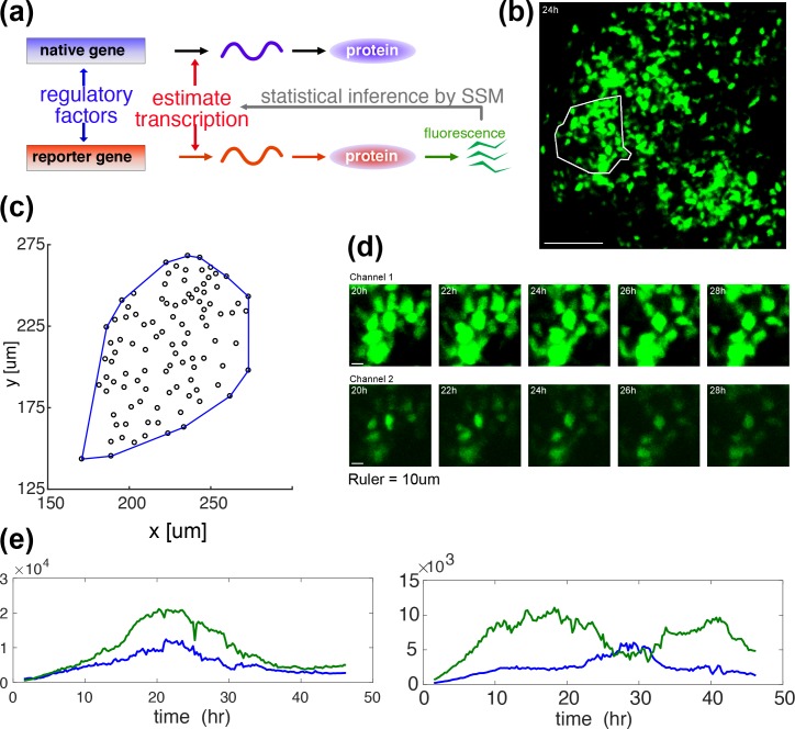
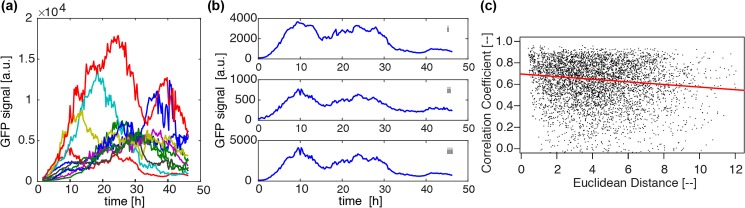
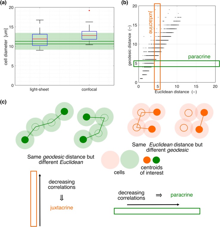
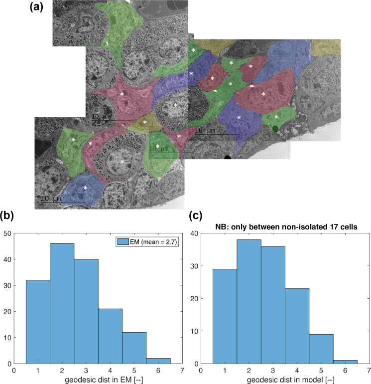
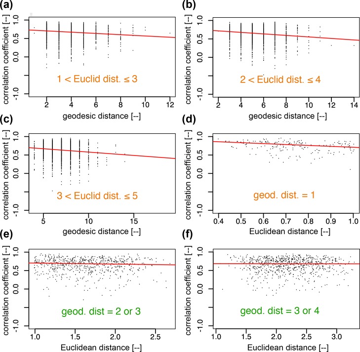
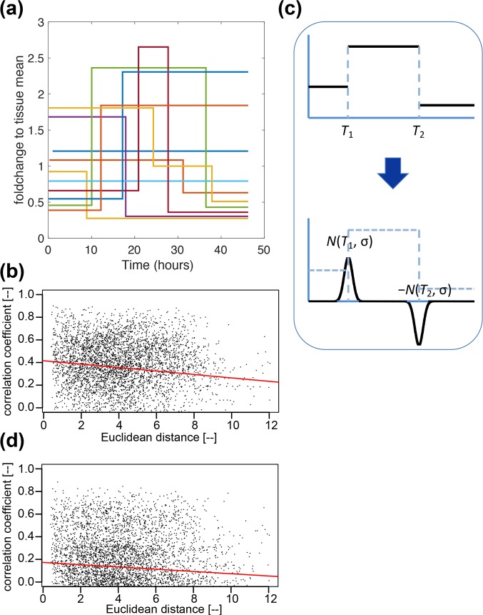
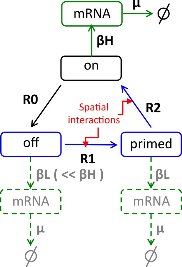
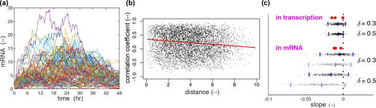
Prolactin is a major hormone product of the pituitary gland, the central endocrine regulator. Despite its physiological importance, the cell-level mechanisms of prolactin production are not well understood. Having significantly improved the resolution of real-time-single-cell-GFP-imaging, the authors recently revealed that prolactin gene transcription is highly dynamic and stochastic yet shows space-time coordination in an intact tissue slice. However, it still remains an open question as to what kind of cellular communication mediates the observed space-time organization. To determine the type of interaction between cells we developed a statistical model. The degree of similarity between two expression time series was studied in terms of two distance measures, Euclidean and geodesic, the latter being a network-theoretic distance defined to be the minimal number of edges between nodes, and this was used to discriminate between juxtacrine from paracrine signalling. The analysis presented here suggests that juxtacrine signalling dominates. To further determine whether the coupling is coordinating transcription or post-transcriptional activities we used stochastic switch modelling to infer the transcriptional profiles of cells and estimated their similarity measures to deduce that their spatial cellular coordination involves coupling of transcription via juxtacrine signalling. We developed a computational model that involves an inter-cell juxtacrine coupling, yielding simulation results that show space-time coordination in the transcription level that is in agreement with the above analysis. The developed model is expected to serve as the prototype for the further study of tissue-level organised gene expression for epigenetically regulated genes, such as prolactin.

Fig 1. GFP imaging in space and time–measurement and representations of prolactin gene transcription.

(a) A diagrammatic illustration of how the GFP reporter measurement is associated with the underlying process of native prolactin gene expression. Expression of the d2EGFP reporter transgene in these studies is controlled by a fragment of the human prolactin gene locus (as described previously[1, 8]). Both the endogenous prolactin gene and the prolactin-d2EGFP reporter gene mRNAs are transcribed in parallel, but are then translated independently into respective proteins (reproduced from [10]). (b) A GFP image of an intact tissue slice from an adult male prolactin-d2EGFP transgenic reporter rat, with a white enclosure to indicate a cell-tracked area for analysis. (c) A spatial distribution of cell centroids, defined as the median over the time-course of the coordinates, with its convex hull (blue). There are 101 cells. The convex hull will be used in Fig 3A in the estimation of the mean cell size. (d) Magnified typical video-frame sequences in time, showing dynamic changes in reporter gene transcription over a collection of single cells. A single sample is recorded concurrently in two channels of high (upper row) and low (lower row) sensitivities. (e) Typical GFP signals in a time course, showing high (left) and low (right) correlations. Correlation coefficients are 0.96 (left) and 0.14 (right) respectively. Each time series obtained in a single cell is reconstructed from two recordings illustrated in (d). See Fig 2B for the reconstruction process.

Fig 2. Properties in network-free analysis in space and time.

(a) GFP time series of ten randomly chosen cells. Time series are reconstructed from two GFP signals recorded simultaneously with different sensitivities to account for saturation effects and to maximise the observed dynamic range. (b) An example of GFP signal reconstruction. Signals from channels 1 (i) and 2 (ii) are combined to restore a linearity between light intensity and GFP reading, yielding a reconstructed signal as in (iii). See Materials and Methods for detailed protocols. (c) Correlation coefficients (Pearson) between GFP time series plotted against Euclidean distance for all cell pairs. The red line shows fit of median regression. Here and throughout the present paper Euclidean distance is normalised by the median cell diameter (see Fig 3A), and is therefore dimensionless. A significant rightward decline, with corresponding p-values shown in S1 Table, is indicative of the presence of space-time coordination in prolactin gene expression profiles.

Fig 3. Cellular network estimation and characterisation of cell pairs by two distance measures.

(a) Box-plots of cell size distributions obtained from light-sheet (left), and confocal (right) micrographs. A red + symbol is an outlier found above the whisker, which is defined to be q3 ± 1.5 (q3—q1), where q1 and q3 are the respective 25th and 75th percentiles. The results are compared to the estimations obtained from the spatial distributions of cell centroids as in Fig 1C (green), with details described in Materials and Methods. With three replicated datasets, the solid horizontal lines represent the means of upper and lower bounds, whose precise definitions are given in Materials and Methods, while the shade is defined by the maximum of the upper bounds and the minimum of the lower bounds. (b) The relationship between Euclidean and geodesic distances for all cell pairs (here and throughout the present paper, Euclidean distance is normalised by the median cell diameter). The latter is a network distance measure, and is defined in detail in Materials and Methods. (c) Schematic illustrations of the cell pairs that are subject to juxtacrine (orange) and paracrine (green) signalling. The cellular network is materialised by their physical contacts. In the orange diagram, geodesic distances are different, 3 on the left and 1 on the right, while Euclidean distances are similar. In the green diagram Euclidean distances are different, larger on the left and small on the right, while the geodesic distance is 3 in both cases. For more details about these two distances, see Materials and Methods (see subsection on Spatial properties in the Computational section). A decreasing correlation with geodesic (Euclidean) distance in a sub-population of cell pairs having a similar Euclidean (geodesic) distance, as illustrated by the enclosed thin orange vertical (green horizontal) rectangle in (b), implies juxtacrine (paracrine) signalling.

Fig 4. Distributions of geodesic distance compared between an electron microscopic (EM) image and the model applied to a GFP image.

(a) A montage of x800 EM images of anterior pituitary tissue, which is different from those GFP imaged (D1, D2, D3). Each lactotroph is shaded in a different colour to distinguish individual cells. There are 18 cells that are fully contained in this montage, and are labelled by *. (b) The distribution of geodesic distance estimated in the EM picture in (a). The 18 cells labelled by * are examined. (c) The distribution of geodesic distance estimated in the model with a GFP dataset. The 18 cells nearest to the tissue centre are examined (see Fig 1C). One cell was found to be isolated from the other 17 cells, causing the histogram y-axis limit smaller than that in (b).

Fig 5. Tests of signalling mechanisms, juxtacrine and paracrine, in the GFP signals.

Juxtacrine signalling is tested in (a)—(c) with geodesic distance (d_G) in the subset of cell pairs that are within a given Euclidean distances (d_E) range, while paracrine signalling is tested in (e)—(f) with Euclidean distances in the subset of cell pairs that have geodesic distances larger than 1. For both signalling modes, a decline to the right in the median regression line suggests the presence of each mode. From the p-values (S1 Table) we conclude the dominance of juxtacrine signalling. The cell pairs characterised by d_G = 1 in (d) are pairs of cells in direct contact. The clear decline in their trend line suggests that the juxtacrine signalling is stronger when there is a larger contact area assuming that, for these cell pairs, greater contact area is correlated with smaller Euclidean distance (i.e. if two cells, each assumed to have a ball shape of a similar diameter, are in contact, the shorter the inter-centroid distance, the larger the contact area).

Fig 6

Analysis of transcriptional profiles inferred by SSM ([7], see also Fig 1(A)). (a) Transcription profiles of ten chosen cells as in Fig 2A. In the SSM their dynamic behaviour is approximated by step functions that have discrete switch points at times around which the transcription rate is estimated to have changed its value given the reporter data. A-priori these rates can take an arbitrary value and are estimated from the reporter data as part of the Bayesian model fitting algorithm described in [7]. (b) The correlations defined using the first score function (Sc1) defined in the text decreases as Euclidean distance increases. Results of statistical tests are in S2 Table, which also summarises the results for juxtacrine and paracrine signalling tested in the transcriptional profiles, showing the dominant presence of juxtacrine signalling as seen for the GFP signals (see Fig 5 and S1 Table). (c) A different representation of transcriptional activity using the second score function (Sc2) defined in the text which puts more emphasis on the timing of the switches than the level of transcription. Each switch is represented by a signed normal distribution with the same amplitude, centred at the switch time, with the same standard deviation being set to 3 hours in reference to ([8], Fig 2Aii). The drop in transcription rate at time T₂ is reflected by a negative sign. (d) Space-time coordination is assessed using median regression of the correlations implied by Sc2 applied to the transformed transcription profiles shown in (c). Scores in these two representations are found to show qualitatively the same behaviour in various signalling tests, as summarised in S2 Table.

Fig 7. A schematic diagram of the model for the transcriptional dynamics in each cell.

The elementary pathway between on, off, and primed is described by a Markov process with an exponential holding time with parameters R_i = 1/t_i. The core of this model is the three cyclic gene states, on, off and primed. The pathways accompanied by R₀, R₁ and R₂ represent the transitions from on to off, from off to primed, and from primed to on, respectively. Conditional on the state we assume that gene expression follows a Markov jump process with birth rates, β_H for on and β_L for off and primed states, and degradation rate μ for mRNA molecules (same for all three states). The values of the rate parameters are found in Materials and Methods. Spatial coupling is implemented by assuming that the rates R₁ and R₂ are a function of the number of on genes in the connected cells (see Eqs (4 and 5) in Materials and Methods).

Fig 8. Simulation results and their correlation analysis.

(a) An example of the mRNA profiles simulated by the model developed above (Fig 7) with parameter values found in Materials and Methods. This set of 108 profiles collectively display a shape that first increases then decreases in time, as in the GFP profiles in experiments (S1 Fig.). (b) Relation between pairwise correlation coefficients and Euclidean distance in the simulation shown in (a) at the mRNA level. (c) Distributions of the estimated slope coefficients (black dots) between the simulated profiles (transcription-rates and mRNA) and Euclidean distance, over 200 simulations. They are accompanied by the blue bars to represent the respective median and the 95% central interval. The distribution at the transcription-rate level is compared to the slopes obtained with the SSM-inferred transcription-rate profiles from the experimental data (three red blobs), while the distribution at the mRNA level is accompanied by the slopes at the GFP level in the same experiments. The grey dots are of the simulations in which the spatial interactions are in action also in the transcription dynamics as defined in Eq (6). This is one possible mechanism that makes the slope of the correlation coefficient in mRNA number steeper. Other potential mechanisms are discussed in the text.

References

1. Harper CV, Finkenstädt B, Woodcock DJ, Friedrichsen S, Semprini S, Ashall L, et al. Dynamic analysis of stochastic transcription cycles. PLoS biology. 2011;9(4):e1000607 10.1371/journal.pbio.1000607 - DOI - PMC - PubMed
1. Spiller DG, Wood CD, Rand DA, White MR. Measurement of single-cell dynamics. Nature. 2010;465(7299):736–45. Epub 2010/06/11. doi: nature09232 [pii] 10.1038/nature09232 . - DOI - PubMed
1. Larson DR. What do expression dynamics tell us about the mechanism of transcription? Current Opinion in Genetics Development. 2011;21(5):591–9. 10.1016/j.gde.2011.07.010 - DOI - PMC - PubMed
1. Suter DM, Molina N, Gatfield D, Schneider K, Schibler U, Naef F. Mammalian genes are transcribed with widely different bursting kinetics. Science. 2011;332(6028):472–4. 10.1126/science.1198817 - DOI - PubMed
1. Coulon A, Chow CC, Singer RH, Larson DR. Eukaryotic transcriptional dynamics: from single molecules to cell populations. Nature Reviews Genetics. 2013;14(8):572 10.1038/nrg3484 - DOI - PMC - PubMed
Publication types