Forget binning and get SMART: Getting more out of the time-course of response data

Abstract

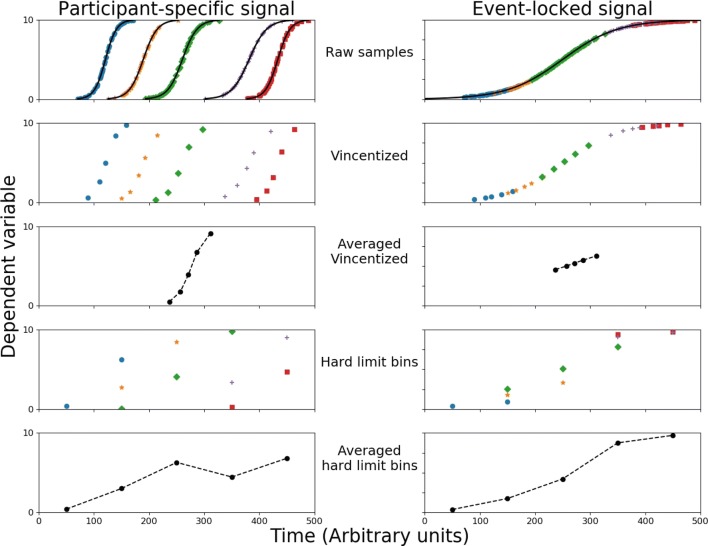
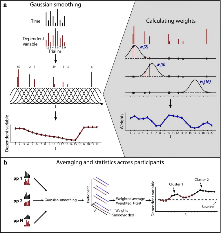
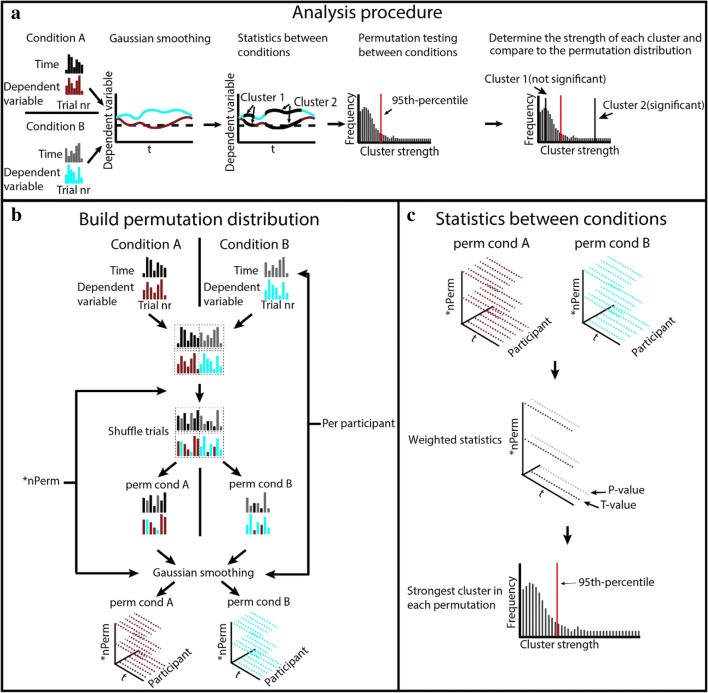
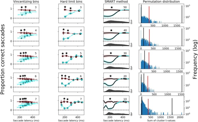
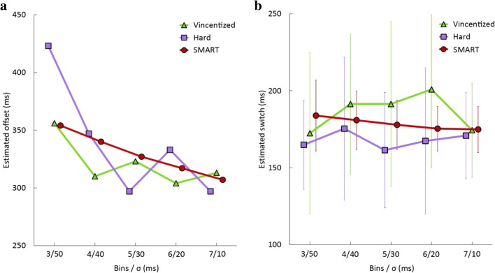
Many experiments aim to investigate the time-course of cognitive processes while measuring a single response per trial. A common first step in the analysis of such data is to divide them into a limited number of bins. As we demonstrate here, the way one chooses these bins can considerably influence the resulting time-course. As a solution to this problem, we here present the smoothing method for analysis of response time-course (SMART)-a complete package for reconstructing the time-course from one-sample-per-trial data and performing statistical analysis. After smoothing the data, the SMART weights the data based on the effective number of data points per participant. A cluster-based permutation test then determines at which moments the responses differ from a baseline or between two conditions. We show here that, in contrast to contemporary binning methods, the chosen temporal resolution has a negligible effect on the SMART reconstructed time-course. To facilitate its use, the SMART method, accompanied by a tutorial, is available as an open-source package.

Keywords: Binning; Perception and action; Reaction time methods; Statistics.

Fig. 1

A simulated dependent variable as a function of time and the reconstruction of the simulated time-course by binning data. The left column shows a simulated dependent variable with a participant-specific signal and responses distributed over the relevant part of the process for each of the five participants. The right column shows a simulated event-locked signal for five participants, but their response-time distributions differ. The panels in both columns, from top to bottom, show raw sample data, per participant Vincentized bins, averaged Vincentized bins, per participant hard-limit bins, and averaged hard-limit bins. Averaged across participants, the time-course of the dependent variable is reconstructed well by Vincentizing for the participant-specific timing, and by hard-limit bins for the event-locked timing. (Color figure online)

Fig. 2

Schematic illustration of the SMART smoothing procedure. a Smoothing for data from one hypothetical participant with nine trials using Eq. 1. Gray insert: Calculating the weight of each smoothed time point for a participant, given by Eq. 2. w_i(t) reflects the sum of kernel density estimates under each Gaussian curve at the sample time point t. b Constructing a weighted average time-course. The data is weighted across participants for each time point. Using Eqs. 3 and 4. The stars reflect the smoothed samples along the time axis. The black stars with connecting black lines equal time points which differ significantly from baseline, given Eq. 5 for testing against a baseline and Eqs. 6 to 8 for paired-sample testing. (Color figure online)

Fig. 3

The SMART analysis procedure. a Procedure overview. b Building the permutation distribution. c Performing statistical analysis and determining significance threshold. (Color figure online)

Fig. 4

Results for Dataset 1. Columns 1–3: The proportion correct saccades as a function of saccade latency when using Vincentizing, hard-limit bins, and SMART, respectively. Cyan indicates the performance of the distractor match condition and dark red indicates the performance of the target match condition. Vertical error bars and shaded areas indicate the 95% confidence intervals. Horizontal error bars indicate the standard deviation of the mean time for each bin across participants. The number in the upper right corner indicates the number of bins or the value for σ. The asterisks in Columns 1 and 2 indicate bins that differ significantly between conditions at p < .05, Bonferroni corrected. In Column 3, the black lines indicate time points at which the two conditions differ significantly from zero, and asterisks indicating which clusters are statistically significant. The dark-gray shaded area is the estimated number of trials per millisecond (right axis), for the target match condition. The light-gray shaded area (completely occluded) is the estimated number of trials per millisecond (right axis) for the distractor match condition. Estimated with the same kernel size as the one used for the SMART procedure. Column 4: The permutation distribution between conditions. The blue histogram shows (on a logarithmic scale) the frequency of the sum of t values of clusters in the permuted time-series. The vertical red line indicates the 95th percentile for the permuted time-series. The vertical black lines indicate the sum of cluster t values in the nonpermuted time-series. (Color figure online)

Fig. 5

Results for Dataset 2. Columns 1–3: Saccade curvature as a function of the intersaccadic interval when using Vincentizing, hard-limit bins and Gaussian smoothing, respectively. The shaded gray area is the estimated number of trials per millisecond (right axis), estimated with the same kernel size as the one used for the SMART procedure. Column 4: The permutation distribution against baseline. Further details as in Fig. 4. (Color figure online)

Fig. 6

The temporal estimates of significant differences in Datasets 1 and 2 as a function of the number of bins (for Vincentized and hard bins) or as a function of the standard deviation (σ) of the Gaussian kernel (for SMART). a The estimated time when the two conditions (target match and distractor match) no longer differ from each other, from Dataset 1. b The estimated saccade curvature switch times, the center point between the borders of the two significant clusters in Fig. 5, from Dataset 2, with error bars reflecting the precision of this estimate (see Method section for details). (Color figure online)

References

1. Boon PJ, Zeni S, Theeuwes J, Belopolsky AV. Rapid updating of spatial working memory across saccades. Scientific Reports. 2018;8(1):1072. doi: 10.1038/s41598-017-18779-9. - DOI - PMC - PubMed
1. Bullmore ET, Suckling J, Overmeyer S, Rabe-hesketh S, Taylor E, Brammer MJ. Global, voxel, and cluster tests, by theory and permutation, for a difference between two groups of structural mr images of the brain. IEEE Transactions on Medical Imaging. 1999;18(1):32–42. doi: 10.1109/42.750253. - DOI - PubMed
1. Fahrenfort JJ, van Leeuwen J, Olivers CNL, Hogendoorn H. Perceptual integration without conscious access. Proceedings of the National Academy of Sciences. 2017;114(14):3744–3749. doi: 10.1073/pnas.1617268114. - DOI - PMC - PubMed
1. Gatz DF, Smith L. The standard error of a weighted mean concentration—I. Bootstrapping vs other methods. Atmospheric Environment. 1995;29(11):1185–1193. doi: 10.1016/1352-2310(94)00210-C. - DOI
1. Godijn R, Theeuwes J. Programming of endogenous and exogenous saccades: Evidence for a competitive integration model. Journal of Experimental Psychology: Human Perception and Performance. 2002;28(5):1039–1054. doi: 10.1037/0096-1523.28.5.1039. - DOI - PubMed