A quantitative confidence signal detection model: 2. Confidence analysis

Abstract

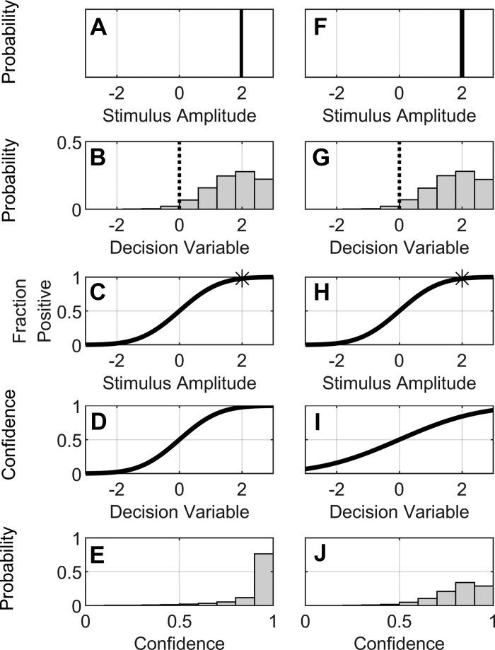
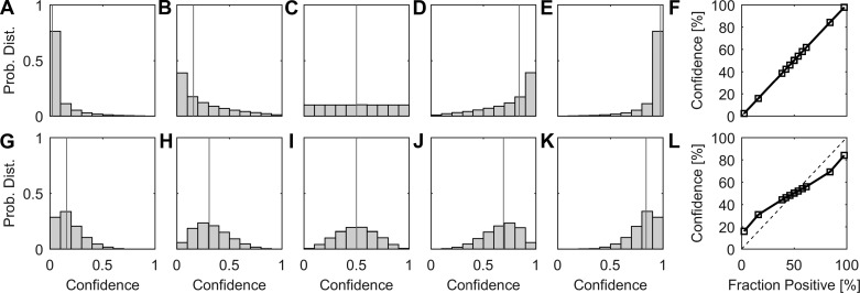
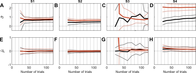
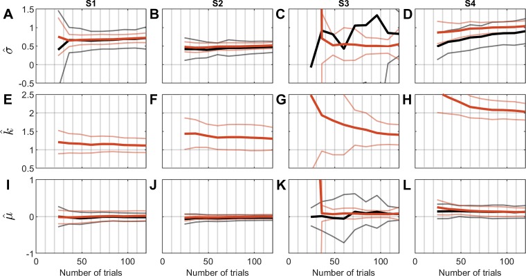
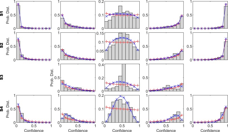
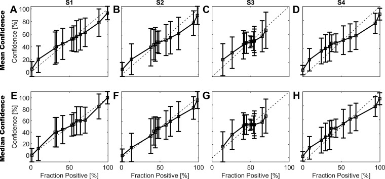
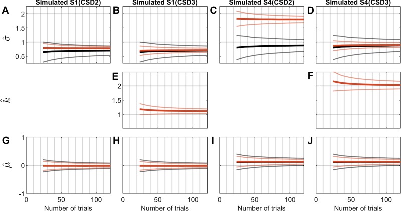
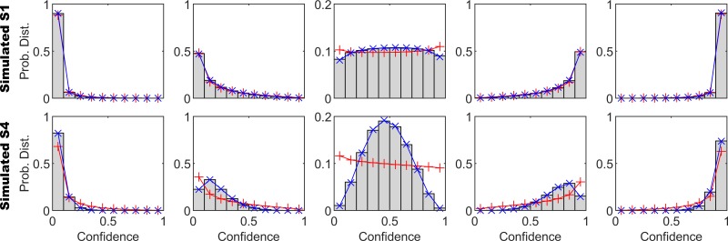
Decision making is a fundamental subfield within neuroscience. While recent findings have yielded major advances in our understanding of decision making, confidence in such decisions remains poorly understood. In this paper, we present a confidence signal detection (CSD) model that combines a standard signal detection model yielding a noisy decision variable with a model of confidence. The CSD model requires quantitative measures of confidence obtained by recording confidence probability judgments. Specifically, we model confidence probability judgments for binary direction recognition (e.g., did I move left or right) decisions. We use our CSD model to study both confidence calibration (i.e., how does confidence compare with performance) and the distributions of confidence probability judgments. We evaluate two variants of our CSD model: a conventional model with two free parameters (CSD2) that assumes that confidence is well calibrated and our new model with three free parameters (CSD3) that includes an additional confidence scaling factor. On average, our CSD2 and CSD3 models explain 73 and 82%, respectively, of the variance found in our empirical data set. Furthermore, for our large data sets consisting of 3,600 trials per subject, correlation and residual analyses suggest that the CSD3 model better explains the predominant aspects of the empirical data than the CSD2 model, especially for subjects whose confidence is not well calibrated. Moreover, simulations show that asymmetric confidence distributions can lead traditional confidence calibration analyses to suggest "underconfidence" even when confidence is perfectly calibrated. These findings show that this CSD model can be used to help improve our understanding of confidence and decision making.NEW & NOTEWORTHY We make life-or-death decisions each day; our actions depend on our "confidence." Though confidence, accuracy, and response time are the three pillars of decision making, we know little about confidence. In a previous paper, we presented a new model - dependent on a single scaling parameter - that transforms decision variables to confidence. Here we show that this model explains the empirical human confidence distributions obtained during a vestibular direction recognition task better than standard signal detection models.

Keywords: confidence calibration; confidence rating; decision making; probability judgments; thresholds; vestibular.

Fig. 1.

Simulated confidence distribution under our signal detection confidence (CSD) model. A: the stimulus for this example is well controlled having an amplitude of +2.0 with little variation, so the objective probability density function is a delta function. B: a signal detection model assumes additive noise. For this example, Gaussian noise having zero-mean and a standard deviation of 1 was simulated ε = N(μ = 0, σ = 1); the distribution for 10,000 samples is shown. The dotted vertical line at zero represents a decision boundary. If a sampled decision variable (d_j) on the jth trial falls to the right of the decision boundary, the subject decides positive. If the sampled decision variable falls to the left, the subject decides negative. For this example, 97.7% of the trials (i.e., decision variables) lead to the subject deciding positive. C: the asterisk, located at (2, 0.977), represents the example data point illustrated in the previous panel. When this process is repeated for a variety of different stimulus levels, it yields a psychometric function, Ψ(x) = φ(x, μ = 0, σ = 1) (black curve). D: the confidence function for a well-calibrated subject (k = 1) is the same as the psychometric function shown in C, χ(x) = Ψ(x). E: the confidence distribution that results from the 10,000 sampled decision variables represented in B. The distribution is calculated by taking each of the 10,000 decision variables represented in B and determining the confidence using the function in D, χ(j) = φ(d_j, μ = 0, kσ = 1). For example, a decision variable of zero would convert to a confidence of 0.5, and decision variable of 2 would convert to a confidence of 0.977. Ordinate for E is truncated at 5 to help illustrate variations. F through J repeat the above process but for an underconfident subject having a confidence-scaling factor of two (k = 2). I shows this underconfidence confidence function, χ(j) = φ(d_j, μ = 0, kσ = 2).

Fig. 2.

Predicted confidence distributions for different models and different stimulus levels. Distributions are calculated using the process outlined in Fig. 1. From left to right, predicted confidence distributions are shown for stimuli equal to −2, −1, 0, 1, and 2, respectively. Top row shows predicted confidence distributions for the exact same noise model ε = N(μ = 0, σ = 1) and confidence function χ(x) = Ψ(x) = ϕ(x, μ = 0, kσ = 1) shown in the left column of Fig. 1. The bottom row shows predicted confidence distributions for the exact same noise model but for an underconfident subject having a confidence-scaling factor of 2 χ(x) = ϕ(x, μ = 0, kσ = 2).

Fig. 3.

Parameter fits for the CSD2 model that fits a psychometric function under a Gaussian noise model, Ψ(x) = ϕ(x, $\widehat{\mu }$, $\widehat{\sigma }$), with the additional assumption that confidence is perfectly calibrated χ(x) = Ψ(x) = ϕ(x, $\widehat{\mu }$, $\widehat{\sigma }$). Each column represents fitted parameters for one of the four subjects (from left to right S1 through S4) in the same order as the previous article (ordered from subject with lowest confidence-scaling factor on left to highest on right). Top row (A–D) shows fitted psychometric width parameter ($\widehat{\sigma }$). Bottom row (E–H) shows fitted psychometric function bias ($\widehat{\mu }$). Thick black curves show average psychometric parameter estimates calculated using conventional forced-choice analyses. Thick red curves show average parameter estimates determined by fitting confidence probability judgment data. Errors bars (thin gray curves and thin red curves, respectively) represent standard deviation of parameter estimates. Data points at 24 (36, 48, . . . 120) trials represent the mean threshold value (across the 30 test sessions) obtained by analyzing data obtained during the first 24 (36, 48, . . . 120) trials for each of the 30 test sessions independently and separately.

Fig. 4.

Parameter fits for the CSD3 model that fits a psychometric function under a Gaussian noise model, Ψ(x) = ϕ(x, $\widehat{\mu }$, $\widehat{\sigma }$) and that simultaneously fits a Gaussian confidence function, χ(x) = ϕ(x, $\widehat{\mu }$, $\widehat{k}\widehat{\sigma }$). Each column represents one of the four subjects in the same order as Fig. 3. Top row (A–D) shows fitted psychometric width parameter ($\widehat{\sigma }$). Middle row (E–H) shows fitted confidence-scaling factor ($\widehat{k}$). Bottom row (I–L) shows fitted psychometric function bias ($\widehat{\mu }$). Thick black curves show average psychometric parameter estimates calculated using conventional forced-choice analyses. Thick red curves show average parameter estimates determined by fitting confidence probability judgment data. Errors bars (thin gray curves and thin red curves, respectively) represent standard deviation of parameter estimates. Data points at 24 (36, 48, . . . 120) trials represent the mean threshold value (across the 30 test sessions) obtained by analyzing data obtained during the first 24 (36, 48, . . . 120) trials for each of the 30 test sessions independently and separately.

Fig. 5.

Confidence probability judgment distributions. Each row represents one of the four subjects (from top to bottom S1 through S4, ordered from subject with lowest confidence-scaling factor on top to highest on bottom). Histograms show empirical human data at each of five stimulus levels. Each column represents different stimulus levels; the largest stimulus magnitudes are represented by the 1st and 5th columns, the 2nd largest stimulus magnitudes are represented by the 2nd and 4th columns, and the remaining relatively small stimuli are represented by the middle (3rd) column. For S3, because the stimuli tested were smaller relative to the actual threshold than for the other three subjects, the 2nd and 4th column show the largest stimulus magnitudes and the center column shows the confidence for remaining subthreshold stimuli. See Table 1 for actual stimulus levels for each subject. Predicted confidence judgment distributions for the CSD2 (red +) and CSD3 (blue x) models using fitted parameters for each subject are overlapped for comparison.

Fig. 6.

Confidence calibration plots. Each column represents one of the four subjects in same order as Fig. 3. Top row shows conventional calibration plots where average confidence for each stimulus level is plotted versus average accuracy. Bottom row shows calibration plots but with median confidence replacing mean confidence. For comparison, Fig. 9 shows similar plots for simulated subjects. Errors bars represent standard deviation.

Fig. 7.

CSD2 and CSD3 parameter fits for simulated subjects S1 and S4. First column shows fitted CSD2 parameters for simulated subject S1. Second column shows fitted CSD3 parameters for simulated subject S1. Third column shows fitted CSD2 parameters for simulated subject S4. Fourth column shows fitted CSD3 parameters for simulated subject S4. Top row (A–D) shows fitted psychometric width parameter ($\widehat{\sigma }$). Middle row (E and F) shows fitted confidence-scaling factor ($\widehat{k}$). Bottom row (G–J) shows fitted psychometric function bias ($\widehat{\mu }$). Thick black curves show average psychometric parameter estimates calculated using conventional forced-choice analyses. Thick red curves show average parameter estimates determined by fitting confidence probability judgment data. Errors bars (thin gray curves and thin red curves, respectively) represent standard deviation of parameter estimates.

Fig. 8.

Simulated confidence probability judgment distributions. Top row shows simulated subject S1. Bottom row shows simulated subject S4. Histograms show simulated data at each of five stimulus levels (−2, −1, 0, 1, 2). Predicted confidence judgment distributions for the CSD2 (red +) and CSD3 (blue ×) models using fitted parameters for each subject are overlapped for comparison.

Fig. 9.

Simulated confidence calibration plots. Errors bars represent standard deviation. First column shows confidence calibration plots for simulated subject S1. Second column shows same confidence data for simulated subject S1 plotted versus stimulus level in a psychometric function plot format where the actual psychometric function is plotted as a dashed curve. Third column shows confidence calibration plots for simulated subject S4. Fourth column shows same confidence data for simulated subject S4 plotted versus stimulus level in a psychometric function plot format where the actual psychometric function is plotted as a dashed curve. Top row shows conventional plots with average confidence plotted versus average accuracy. For bottom row, median confidence replaces mean confidence for y-axis of all four subplots.

References

1. Balakrishnan JD, Ratcliff R. Testing models of decision making using confidence ratings in classification. J Exp Psychol Hum Percept Perform 22: 615–633, 1996. doi:10.1037/0096-1523.22.3.615. - DOI - PubMed
1. Benson AJ, Hutt EC, Brown SF. Thresholds for the perception of whole body angular movement about a vertical axis. Aviat Space Environ Med 60: 205–213, 1989. - PubMed
1. Benson AJ, Spencer MB, Stott JR. Thresholds for the detection of the direction of whole-body, linear movement in the horizontal plane. Aviat Space Environ Med 57: 1088–1096, 1986. - PubMed
1. Björkman M, Juslin P, Winman A. Realism of confidence in sensory discrimination: the underconfidence phenomenon. Percept Psychophys 54: 75–81, 1993. doi:10.3758/BF03206939. - DOI - PubMed
1. Brier GW. Verification of forecasts expressed in terms of probability. Mon Weather Rev 78: 1–3, 1950. doi:10.1175/1520-0493(1950)078<0001:VOFEIT>2.0.CO;2. - DOI
Publication types
LinkOut - more resources