The resonant brain: How attentive conscious seeing regulates action sequences that interact with attentive cognitive learning, recognition, and prediction

Abstract

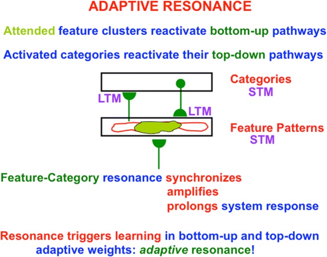
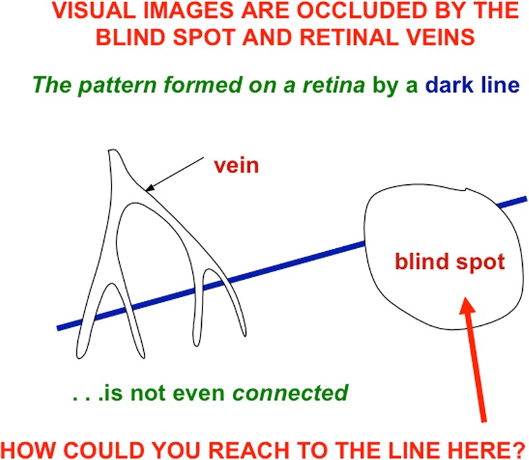
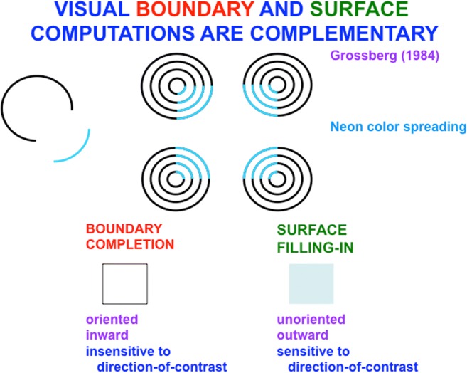
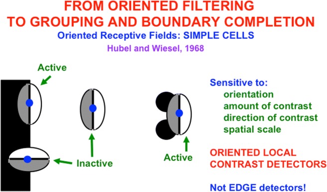
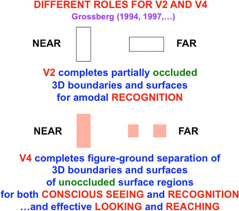
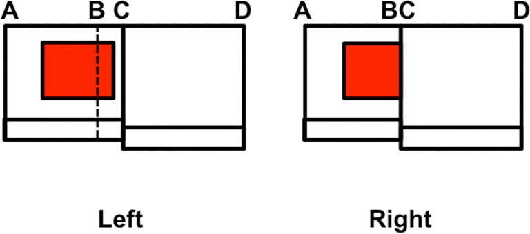
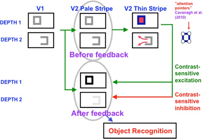
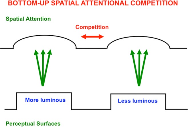
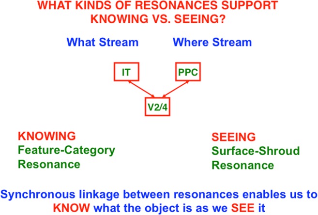
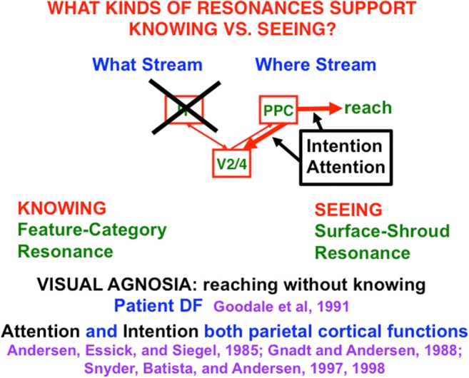
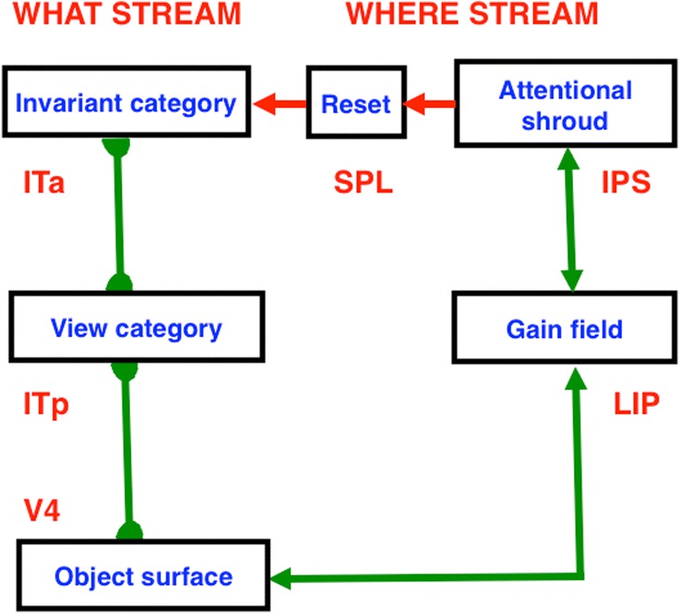
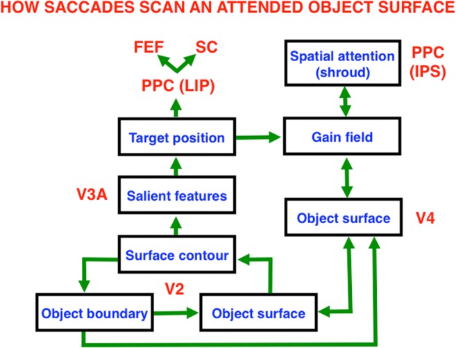
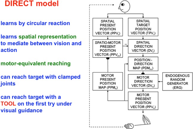
This article describes mechanistic links that exist in advanced brains between processes that regulate conscious attention, seeing, and knowing, and those that regulate looking and reaching. These mechanistic links arise from basic properties of brain design principles such as complementary computing, hierarchical resolution of uncertainty, and adaptive resonance. These principles require conscious states to mark perceptual and cognitive representations that are complete, context sensitive, and stable enough to control effective actions. Surface-shroud resonances support conscious seeing and action, whereas feature-category resonances support learning, recognition, and prediction of invariant object categories. Feedback interactions between cortical areas such as peristriate visual cortical areas V2, V3A, and V4, and the lateral intraparietal area (LIP) and inferior parietal sulcus (IPS) of the posterior parietal cortex (PPC) control sequences of saccadic eye movements that foveate salient features of attended objects and thereby drive invariant object category learning. Learned categories can, in turn, prime the objects and features that are attended and searched. These interactions coordinate processes of spatial and object attention, figure-ground separation, predictive remapping, invariant object category learning, and visual search. They create a foundation for learning to control motor-equivalent arm movement sequences, and for storing these sequences in cognitive working memories that can trigger the learning of cognitive plans with which to read out skilled movement sequences. Cognitive-emotional interactions that are regulated by reinforcement learning can then help to select the plans that control actions most likely to acquire valued goal objects in different situations. Many interdisciplinary psychological and neurobiological data about conscious and unconscious behaviors in normal individuals and clinical patients have been explained in terms of these concepts and mechanisms.

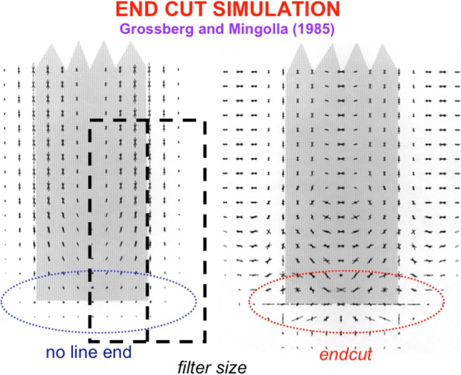
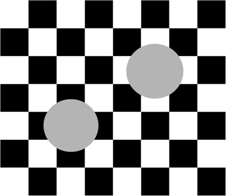
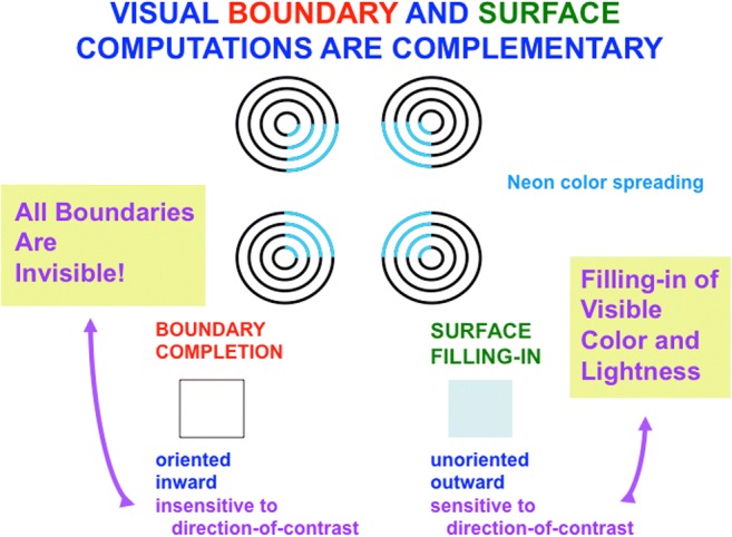
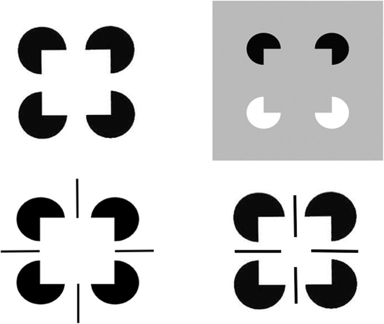
Keywords: Adaptive resonance; Arm movement; Boundary completion; Cognitive plan; Cognitive working memory; Complementary computing; Consciousness; Feature–category resonance; Figure–ground separation; Hierarchical resolution of uncertainty; IPS; Invariant object category learning; LIP; Movement sequences; Neon color spreading; Object attention; PFC; PPC; Saccadic eye movement; Spatial attention; Surface filling-in; Surface–shroud resonance; V2; V3A; V4.

Fig. 1

During an adaptive resonance, attended feature patterns interact with recognition categories, both stored in short-term memory (STM), via positive feedback pathways that can synchronize, amplify, and prolong the resonating cell activities. Such a resonance can trigger learning in the adaptive weights, or long-term memory (LTM) traces, within both the bottom-up adaptive filter pathways and the top-down learned expectation pathways. In the present example, the resonance is a feature–category resonance (see Table 1a). (Color figure online)

Fig. 2

This image emphasizes that, even the retinal image of a simple object like a line can be occluded in multiple places by retinal veins and the blind spot, thereby creating multiple positions along the line that do not provide reliable inputs to the brain for directing actions to those positions. (Color figure online)

Fig. 3

Simplified schematic of the anatomy of three processing streams in the visual cortex. The LGN-blob-(thin stripe)-V4 stream fills-in visual surfaces, whereas the LGN-interblob-interstripe-V4 stream completes visual boundaries. LGN = lateral geniculate nucleus; V1 = striate visual cortex; V2, V3, V4, MT = prestriate cortical areas. The motion stream goes through V1 and MT to the parietal areas. Reproduced with permission from DeYoe and van Essen (1988). (Color figure online)

Fig. 4

An example of neon color spreading. The image consists of black and blue circular arcs. The percept of the color blue filling a square is a visual illusion that is constructed by the brain. The process whereby boundaries are completed are computationally complementary to the process whereby surfaces fill-in brightness, color, and depth. See the text for details. (Color figure online)

Fig. 5

A network of simple, complex, and hypercomplex cells begins the processing of perceptual boundaries. Pairs of like-oriented simple cells with opposite contrast polarity selectivities at each position add their inputs to complex cells. Complex cells input to hypercomplex cells through a short range spatial competition (1st), followed by an orientational competition at each position (2nd). The spatial competition can cause end gaps in boundaries. The orientational competition can cause end cuts in boundaries. The hypercomplex cells in the second competitive stage input to cooperative bipole grouping cells. (Color figure online)

Fig. 6

Simple cells are oriented local contrast detectors that are sensitive to the position, orientation, amount and direction of contrast, and size of visual stimuli. They are not just edge detectors, but can rather response to oriented edges, shading, and texture. (Color figure online)

Fig. 7

Although simple cells with the proper contrast polarity and orientational selectivity can respond to all sides of a sufficiently thick bar, they cannot respond to the ends of sufficiently thin lines. For each spatial scale of a simple cell, one can construct a range of line widths that has this property. The red lines represent the positions and orientations of the simple cell responses to the bar and line end in the image. (Color figure online)

Fig. 8

The missing boundary at the bottom of the line end is completed by an end cut. The brain network that does this needs to be sensitive to the pattern of activations near the line end, not just to the responses or nonresponses of cells to individual positions, or pixels. Otherwise, the brain would be faced with the impossible task of creating something (an end cut) out of nothing (the nonresponse at the line end). (Color figure online)

Fig. 9

The left image shows a computer simulation of the responses of model complex cells to a line end. The line end is shown in gray. The spatial scale of the cells is shown by the dark hatched double-rectangular region. The magnitude of an oriented cell’s response at each position is proportional to the length of the line drawn with the same orientation at that position. Note that, although strong vertical and nearly vertical responses occur along and near the sides of the line, there are no responses at the line end. The right image shows the end cut that is created at the hypercomplex cells by inputs from these complex cell responses. Note that the end cut is positionally hyperacute but orientationally fuzzy. The latter property enables end cuts to form parts of groupings that are perpendicular and nearly perpendicular to line ends, as in the percept of neon color spreading in Fig. 4. Adapted with permission from Grossberg and Mingolla (1985).(Color figure online)

Fig. 10

As the circumferences of the two disks are traversed, the relative contrast reverses periodically, from dark-to-light (gray-to-white) to light-to-dark (gray-to-black) and back again. Although simple cells that are sensitive to one contrast polarity could not form a boundary around the entire circumference of these disks, hypercomplex cells can. This image also creates a strong amodal percept that the upper right disk occludes a white cross, whereas the lower left disk occludes a black cross. These percepts violate a Bayesian account of the most probable percept that an occluded checkerboard lies behind these gray disks

Fig. 11

Neon color spreading illustrates computationally complementary properties of boundary completion and surface filling in, notably that all boundaries are invisible, and that visible qualia are surface percepts. (Color figure online)

Fig. 12

The image in the upper row (left) is a Kanizsa square. The illusory square looks brighter than its background and in front of four partially occluded disks whose unoccluded parts have the shape of Pac-Man figures. See Grossberg (2014) for an explanation of how the apparent brightness and depth of the emergent square covary. The image in the upper row (right) is a reverse-contrast Kanizsa square. The illusory square can be recognized, but many people do not see it because the filled-in gray colors inside and outside the square are approximately equal. This is due to the fact that there are two white Pac-Men and two black Pac-Men on a gray background. The white Pac-Men cause darker feature contours within the illusory square, whereas the black Pac-Men cause brighter feature contours within the illusory square. When these darker and brighter feature contours fill in within the square, they tend to cancel out. The same thing happens outside the square. The net effect is a similar gray color both inside and outside the square. The square thus can be recognized, but not seen. In the lower row, two Kanizsa square percepts are generated using additional lines that either abut the emergent square boundary or penetrate it, leading to dramatically different percepts. (Color figure online)

Fig. 13

Even the straight line in Fig. 2 can be occluded in multiple positions by the blind spot and retinal veins (top image). To complete the occluded representation in the top image of this figure, both boundary completion (middle image) and surface filling-in (bottom image) are needed

Fig. 14

Bipole cell properties in cortical area V2 were first reported by von der Heydt, Peterhans and Baumgartner (1984). The various cases of cell response and nonresponse, as recorded at the probe location, clarify that, either direct activation of the cell at the probe location, or approximately like-oriented input stimuli to both branches, or “poles,” of the cell’s receptive field, are needed to fire the cell, and this continues to be true if the positions of these oriented inputs are moved back and forth within these branches

Fig. 15

(Left panel) The bipole cell receptive field enables multiple nearby orientations and positions to initiate grouping. (Right panel) Despite this initially coarse grouping, the final grouping is often sharp in both its positional and orientational selectivity due to feedback interactions within the entire network

Fig. 16

(Top row) A closed boundary contour (in blue) surrounds a pattern of illuminant-discounted feature contour activities (in red) before filling-in occurs. (Middle row, left column) After filling-in within the closed boundary, the filled-in activity spreads through the entire surface region within the rectangular closed boundary. (Middle row, right column) If there is a large hole, or gap, in a boundary, then color can flow out of it and equalize the filled-in surface activity on both sides of the boundary. Because of this difference, closed and open boundaries are processed differently during figure–ground separation. (Bottom row) Output signals form along the bounding contour of a filled-in surface that is surrounded by a closed boundary. The activity of cells in this surface contour is greater at the positions of salient features like the corners of the rectangle. (Color figure online)

Fig. 17

(Left column) Three abutting rectangles cause a compelling percept of a vertical bar that partially occludes a horizontal bar. (Right column) The occluded region of the horizontal bar is amodally recognized without being consciously seen. If all such completed occluded regions could be seen, then all occluders would look transparent. Interactions between cortical areas V2 and V4 are predicted to prevent this from happening. See the text for details about how this is proposed to happen

Fig. 18

Whereas cortical area V2 is predicted to complete depth-selective amodal boundary and surface representations of the bars in Fig. 17 for purposes of recognition, cortical area V4 is predicted to fill-in depth-selective unoccluded surface regions for conscious seeing and recognition, and for looking and reaching

Fig. 19

An example of a simple scene that illustrates da Vinci stereopsis, as seen through the left (L) and right (R) eyes in depth. See the text for details

Fig. 20

Surface contour signals ensure complementary consistency of boundaries and surfaces while also initiating figure–ground separation. The filled-in surface color or brightness of a region that is surrounded by a closed boundary (at Depth 1 of V2 thin stripes) can generate surface contour signals at the positions of that boundary. These surface contour signals strengthen the boundaries that induced the surface (at Depth 1 of V2 pale stripes), while inhibiting the spurious boundary signals at the same positions, but further depths (at Depth 2 of V2 pale stripes). With these spurious boundaries eliminated, partially occluded objects (not shown) can be amodally completed at the further depth plane (Depth 2) via collinear bipole boundary completion. A percept of two figures, one partially occluding another, can thereby be generated, as in response to the image in Figure (left column)

Fig. 21

A cross-section of a simple filled-in surface (e.g., in cortical area V4) is shown in which a more contrastive bar is to the left of a less contrastive bar. Each position in the surface sends topographic bottom-up excitatory signals to the spatial attention region (e.g., PPC) where the activated cells compete

Fig. 22

Each activated spatial attention cell sends topographic top-down excitatory signals to the corresponding surface, while it also sends broad off-surround inhibitory signals to other spatial attention cells, thereby activating a recurrent on-center off-surround network whose cells obey shunting laws. This recurrent network generates a surface–shroud resonance that contrast-enhances the more active spatial attention cells, while inhibiting the less active ones, thereby creating a form-sensitive distribution of spatial attention, or attentional shroud, that focuses spatial attention upon the more contrastive surface, while also increasing its effective contrast

Fig. 23

Seeing and knowing. A surface–shroud resonance that supports conscious seeing and a feature–category resonance that supports conscious knowing, or recognition, can occur simultaneously and be supported by a synchronous resonance that bridges the “what” and “where” cortical streams via shared prestriate visual cortical circuits

Fig. 24

When a feature–category “knowing” resonance is lesioned, the corresponding surface–shroud “seeing” resonance can still trigger an action, as occurs during visual form agnosia. This figure also diagrams the distinction between the roles of PPC in controlling top-down spatial attention versus the intention to move

Fig. 25

Learning of view-invariant categories in the “what” cortical stream is regulated by surface–shroud resonances in the “where” cortical stream. The surface–shroud resonance between V4 and IPS maintains sustained spatial attention upon an object surface at the same time that it prevents an emerging invariant category in ITa from being reset as multiple view-specific categories in ITp are learned and associated with it as the eyes scan the attended object surface. See the text for details

Fig. 26

This circuit summarizes some of the key cortical processing stages that help to control sequences of saccadic eye movements that are directed to salient features of an attended object surface. See the text for details

Fig. 27

DIrection-to-Rotation Effector Control Transform, or DIRECT, model circuit mechanisms: An endogenous random generator, or ERG, energizes motor learning during a critical period of motor babbling. The ERG activates a motor direction vector (DVm) that moves the hand/arm via the motor present position vector (PPVm). As the hand/arm moves, the eyes reactively track the position of the moving hand, and compute a visually activated spatial target position vector (TPVs) and a spatial present position vector (PPVs). These vectors coincide during reactive tracking. Together they compute the spatial difference vector (DVs). This spatial computation, together with the mapping from spatial directions into motor directions, is the basis of motor-equivalent reaching properties. To compute them, the PPVs activates the spatiomotor present position vector (PPVsm), which is subtracted from the TPVs. Because the PPVs signal to the TPVs is slightly delayed, DVs can be computed. The PPVsm stage is one of two model stages where spatial (s) and motor (m) representations combine. A circular reaction (Piaget, 1945, 1951, 1952), is learned from spatial-to-motor and motor-to-spatial representations at the two adaptive pathways denoted by hemispherical synapses. The spatial direction vector (DVs) is hereby adaptively mapped into the motor direction vector (DVm) to transform visual direction into joint rotation. Adapted with permission from Bullock, Grossberg, and Guenther (1993)

References

1. Andersen RA, Brotchie PR, Mazzoni P. Evidence for the lateral intraparietal area as the parietal eye field. Current Opinion in Neurobiology. 1992;2:840–846. - PubMed
1. Andersen RA, Essick GK, Siegel RM. Encoding of spatial location by posterior parietal neurons. Science. 1985;230:456–458. - PubMed
1. Andersen RA, Essick GK, Siegel RM. Neurons of area 7 activated by both visual stimuli and oculomotor behavior. Experimental Brain Research. 1987;67:316–322. - PubMed
1. Andersen RA, Mountcastle VB. The influence of the angle of gaze upon the excitability of the light- sensitive neurons of the posterior parietal cortex. Journal of Neuroscience. 1983;3:532–548. - PMC - PubMed
1. Andersen RA, Snyder LH, Batista AP, Buneo CA, Cohen YE. Posterior parietal areas specialized for eye movements (LIP) and reach (PRR) using a common coordinate frame. In: Bock GR, Goode JA, editors. Sensory guidance of movement (Novartis Foundation Symposium 218) Chichester, UK: Wiley; 1998. pp. 109–128. - PubMed
LinkOut - more resources