. 2019 Aug 7;103(3):520-532.e5.
doi: 10.1016/j.neuron.2019.05.032. Epub 2019 Jun 20.

Transforming the Choice Outcome to an Action Plan in Monkey Lateral Prefrontal Cortex: A Neural Circuit Model

Affiliations

Transforming the Choice Outcome to an Action Plan in Monkey Lateral Prefrontal Cortex: A Neural Circuit Model

Man Yi Yim et al. Neuron. .

Abstract

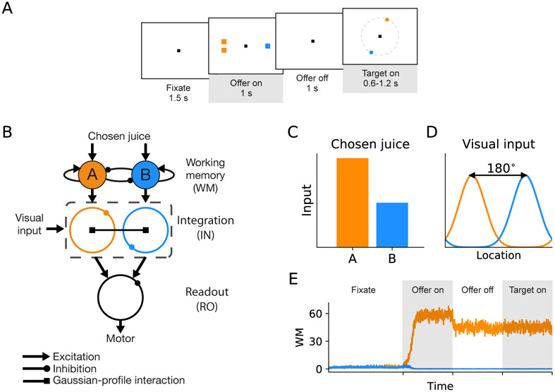
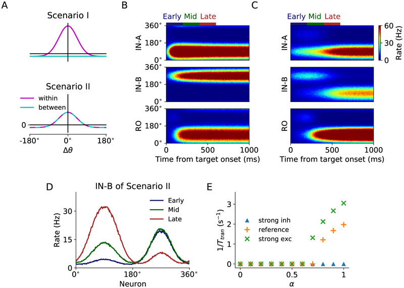
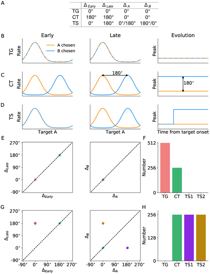
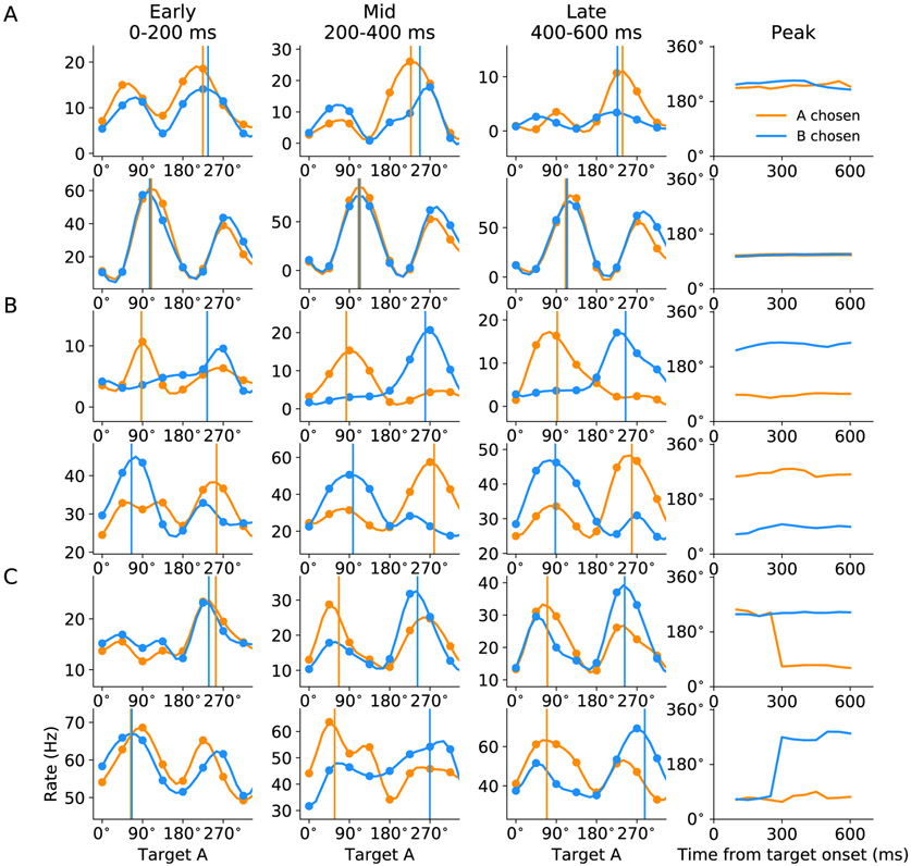
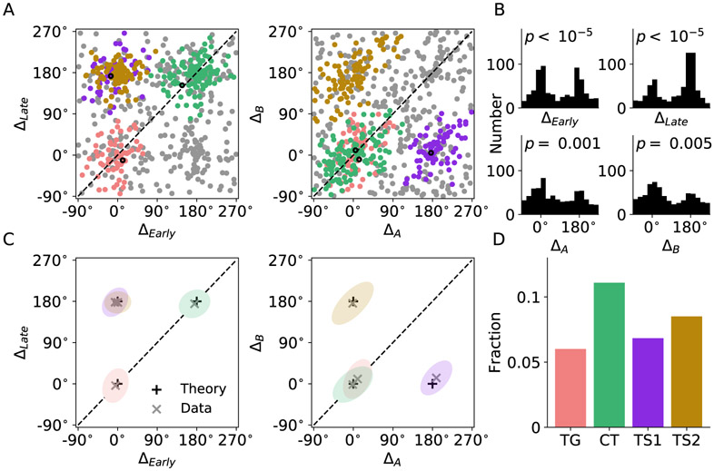
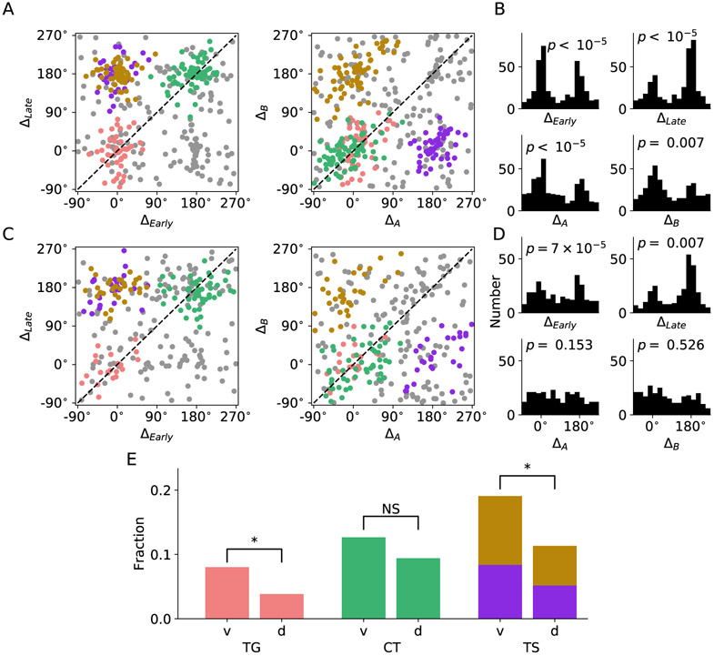
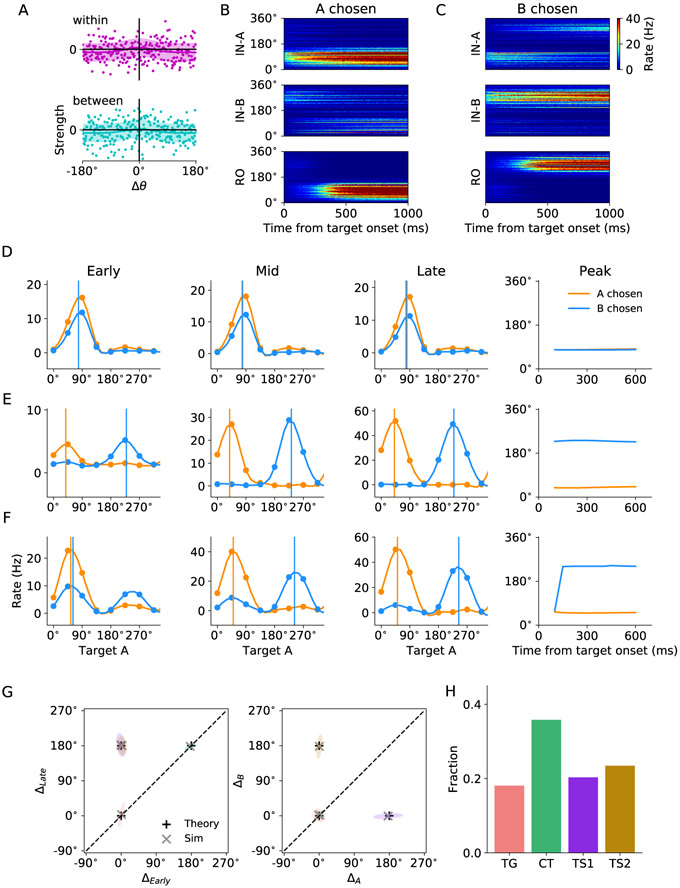
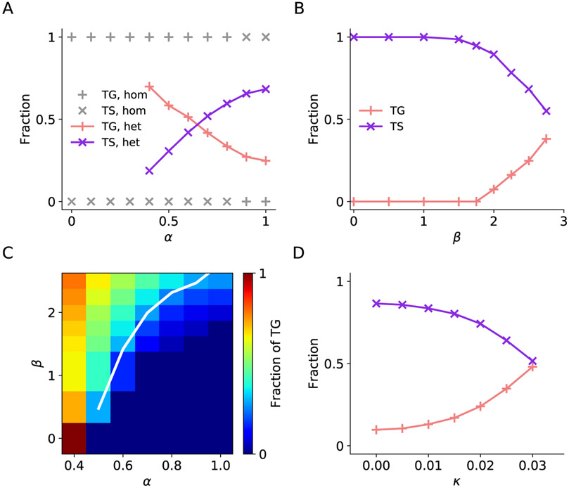
In economic decisions, we make a good-based choice first, then we transform the outcome into an action to obtain the good. To elucidate the network mechanisms for such transformation, we constructed a neural circuit model consisting of modules representing choice, integration of choice with target locations, and the final action plan. We examined three scenarios regarding how the final action plan could emerge in the neural circuit and compared their implications with experimental data. Our model with heterogeneous connectivity predicts the coexistence of three types of neurons with distinct functions, confirmed by analyzing the neural activity in the lateral prefrontal cortex (LPFC) of behaving monkeys. We obtained a much more distinct classification of functional neuron types in the ventral than the dorsal region of LPFC, suggesting that the action plan is initially generated in ventral LPFC. Our model offers a biologically plausible neural circuit architecture that implements good-to-action transformation during economic choice.


Figures

Figure 1.
Figure 1.. Task design and basic structure of neural circuit model.
(A) The neural circuit model was constructed based on the behavioral task in Cai and Padoa-Schioppa (2014). At the beginning of the trial, the monkey fixated a center point on the monitor. After 1.5 s, two offers appeared to the left and right of the fixation point. The offers were represented by sets of color squares, with the color indicating the juice type and the number of squares indicating the juice amount. The offers remained on the monitor for 1 s, and then they disappeared. The monkey continued fixating for another 1 s, after which two saccade targets appeared. The location of the saccade targets was randomly selected on a circle centered on the fixation point out of eight possible locations, with the two saccade targets on opposite sides of the fixation point. The saccade targets were of different colors corresponding to the colors of the two juices. The monkey maintained fixation for an additional randomly variable delay (0.6-1.2 s) before the center fixation point was extinguished, which served as the “go” signal. (B) Schematic of the circuit model. The working memory (WM) neuronal population in LPFC receives chosen juice input. The integration (IN) neuronal population integrate visual input from sensory areas and chosen juice input from WM. Finally, IN population project to readout (RO) population where the chosen target output is sent to the downstream motor area(s). A filled circle and a ring represent a population of homogeneous neurons and a ring network, respectively. Different types of arrows stand for different types of synaptic interaction, as specified below the circuit schematic.(C) The chosen juice input is presented during offer on period as currents of different amplitudes.(D) The visual input is presented as a Gaussian-profiled current which peaks at the direction of the target cue. Note that the two target cues are always opposite to each other, that is, 180° apart.(E) Activity profile of the WM module when A is the chosen juice, which exhibits the typical winner-take-all attractor dynamics. The shaded time intervals correspond to offer on and target on periods shown in (A).
Figure 2.
Figure 2.. Model scenarios and circuit dynamics.
(A) Model scenarios and circuit dynamics for Scenario I and II. In Scenario I (α = 0)the interaction within rings follows a Gaussian spatial profile, while the interaction between rings has no spatial dependence. In Scenario II (α = 1), the interaction within and between rings follows the same Gaussian profile. The total synaptic weight within the dual-ring network is conserved in both scenarios. (B) Scenario I: spatiotemporal activity pattern of IN and RO population of the circuit model from target onset when the chosen target is A, presented at 90°. (C) Same as (B) but for Scenario II. Note that there is a 180° transition of the activity bump in IN-B ring during 200 – 400 ms after target onset. (D) Activity profile of IN-B ring of Scenario II in different time windows. Early, mid and late time windows are defined at 0 – 200 ms, 200 – 400 ms and 400 — 600 ms, respectively, after target onset. The activity bump initially appears at 270°, but then another bump at chosen target location 90° grows over time and the initial bump is suppressed. (E) Effect of between-IN ring excitatory interaction on transition time. We consider three conditions: strong inhibition (J = −0.6 nA, J+ = 1.9 nA), reference (J = −0.35 nA, J+ = 1.9 nA) and strong overall excitation (J = −0.35 nA, J+ = 2.02 nA). When inhibition is strong, no transition occurs. When excitation is sufficiently strong, transition takes place at large α. The stronger the excitation and the larger the value of α, the earlier the transition occurs, giving rise to a larger inversed transition time.
Figure 3.
Figure 3.. Model predictions of functional neuron types.
(A) Peak differences for the three functional types of neurons according to the model. The four independent peak differences are defined to characterize the spatial tuning of every neuron during good-to-action transformation (see EXPERIMENTAL PROCEDURES). Note that the peak location of spatial tuning curves is identified with respect to target A location. TG neurons encode the location of the associated target throughout a trial, independent of whether A or B is chosen, therefore all peak differences are 0°. CT neurons carry the chosen target signal throughout, that is, ΔA = ΔB = 0°, whereas the peak differences between the two tuning curves at different time intervals are 180°. TS neurons behave like TG in the early stage and like CT in the late stage. If a TS neuron is in ring A, its peak location for chosen juice A is constant over time, giving rise to ΔA = 0° (D, orange) while its peak location for chosen juice B experiences a 180° change (D, blue). Vice versa for a TS neuron in ring B. Therefore, a TS neuron will take up one of the two locations in the 4-dimensional space of peak difference. (B-D) Left: Spatial tuning curves contingent upon the identity of chosen juice for units in the model categorized asTG, CT and TS neurons. Right: Time evolution of the peak location of the spatial tuning curves of the three neuron types. (E) Representation of neurons in space of peak difference according to Scenario I. The 4-dimensional space was decomposed into two 2-dimensional subspaces. Note that the representations of TG and CT neurons overlap in the subspace ΔA versus ΔB (F) Number of different neuron types according to Scenario I. (G) Representation of neurons according to Scenario II as in (E). Note that the representations of TS1 and TS2 neurons overlap in the subspace ΔEarly versus ΔLate. (H) Number of different neuron types according to Scenario II.
Figure 4.
Figure 4.. Examples of the three neuron types from LPFC.
Spatial tuning curves and time evolution of their peak location of two putative (A) TG neurons, (B) CT neurons, (C) TS neurons. The tuning curves were constructed by cubic spline interpolation.
Figure 5.
Figure 5.. LPFC neuron type classification.
(A) Representation of spatially selective neurons in the space of peak differences. The clusters were detected with DBSCAN. Different clusters were represented by different colors with gray as unclassified. The first example neuron of each functional type in Figure 4 is marked with a black circle. (B) Histograms for each dimension. The p-values indicate the significance of the dip test. (C) Representation of neuron clusters in peak-difference space. Each ellipse represents one SEM of one cluster. Black pluses indicate theoretically predicted locations of peak differences for different neuron types, while gray crosses denote the center (mean) for each cluster, which are also the centers of the ellipses. (D) Fraction of different neuron types among all the recorded LPFC neurons.
Figure 6.
Figure 6.. LPFC neuron type classification.
Spatially selective neurons in Figure 5C were plotted separately for LPFCv and LPFCd. (A) Representation of LPFCv neurons in the space of peak-difference. (B) Histograms of LPFCv neuron count for each dimension of peak-difference. (C) Same as (A) but for LPFCd. (D) Same as (B) but for LPFCd. (E) Fraction of different neuron types among all recorded neurons in LPFCv and LPFCd. Asterisks indicate significant difference in fraction (p < 0.05, two-sample t-test).
Figure 7.
Figure 7.. Effects of heterogeneity in network interactions on the properties of the circuit model in Scenario III.
(A) An example of interaction profiles within (top) and between (bottom) IN rings for one neuron in the ring. The mean interaction strength has a Gaussian profile and the shaded boundaries correspond to one standard deviation. (B) Activity of model neurons when target A which appeared at 90° was chosen. (C) Activity of model neurons when target B which appeared at 270° was chosen. (D-F) Spatial tuning curves and time evolution of their peak location of a TG neuron (D), CT neuron and TS neuron (F). The tuning curves were constructed by cubic spline interpolation. (G) Representation of neuron clusters in peak-difference space. Each ellipse represents one SEM of one cluster. Black pluses indicate theoretically predicted locations of peak differences for different neuron types, while gray crosses denote the mean for each cluster, or the center of the ellipse. (H) Fraction of different neuron types.
Figure 8.
Figure 8.. Effects of synaptic interactions on quantitative predictions of neuron types.
(A) Fraction of TG and TS neurons in the two IN rings as a function of between-ring excitatory interaction strength α for homogeneous network (β = 0, gray) and heterogeneous network (β = 2.5 nA, colored). Heterogeneity in network interactions gives rise to the coexistence of TG and TS neurons in the two rings. Larger α favors the existence of TS neurons. (B) Fraction of TG and TS neurons as a function of standard deviation of excitatory interaction strength β at α = 0.9. Higher level of heterogeneity, as indicated by higher β value, favors the existence of TG neurons at large α. (C) Fraction of TG neurons as a function of α and β. The white line indicates the fraction of TG neurons equal to 0.28, the fraction observed in experiment. (D) Fraction of TG and TS neurons as the intrinsic neuronal heterogeneity κ varies. Here neuronal heterogeneity is implemented by drawing two Gaussian-distributed parameters for each neuron. α and β were set to be 0.9 and 2 nA, respectively. Higher level of neuronal heterogeneity, as indicated by higher κ value, favors the existence of TG neurons.

Similar articles

Cited by

References

    1. Abbott L, and Chance FS (2005). Drivers and modulators from push-pull and balanced synaptic input. Prog. Brain Res 149, 147–155. - PubMed
    1. Ardid S, and Wang XJ (2013). A tweaking principle for executive control: neuronal circuit mechanism for rule-based task switching and conflict resolution. J. Neurosci 33, 19504–17. - PMC - PubMed
    1. Asplund CL, Todd JJ, Snyder AP, and Marois R (2010). A central role for the lateral prefrontal cortex in goal-directed and stimulus-driven attention. Nat. Neurosci 13, 507–512. - PMC - PubMed
    1. Ben-Yishai R, Bar-Or RL, and Sompolinsky H (1995). Theory of orientation tuning in visual cortex. Proc. Natl. Acad. Sci. U.S.A 92, 3844–8. - PMC - PubMed
    1. Berens P (2009). CircStat : a MATLAB toolbox for circular statistics. J. Stat. Softw 31, 1–21.

Publication types

LinkOut - more resources