High-dimensional geometry of population responses in visual cortex

Abstract

A neuronal population encodes information most efficiently when its stimulus responses are high-dimensional and uncorrelated, and most robustly when they are lower-dimensional and correlated. Here we analysed the dimensionality of the encoding of natural images by large populations of neurons in the visual cortex of awake mice. The evoked population activity was high-dimensional, and correlations obeyed an unexpected power law: the nth principal component variance scaled as 1/n. This scaling was not inherited from the power law spectrum of natural images, because it persisted after stimulus whitening. We proved mathematically that if the variance spectrum was to decay more slowly then the population code could not be smooth, allowing small changes in input to dominate population activity. The theory also predicts larger power-law exponents for lower-dimensional stimulus ensembles, which we validated experimentally. These results suggest that coding smoothness may represent a fundamental constraint that determines correlations in neural population codes.

Extended Data Fig. 1. Reliability of single neuron responses.

a, A single neuron’s response to the first repeat of 2800 stimuli plotted against its responses to the second repeat of the same stimuli. b, Histograms of p-values for Pearson correlation of responses on the two repeats. Each colored histogram represents a different recording. 81.4 ± 5.1% (SE, n=7 recordings) of cells were significant at p<0.05. c, Histogram of the single neuron percentage of stimulus-related variance across the population. Each colored histogram represents a different recording; arrowheads (top) represent the mean for each experiment.

Extended Data Fig. 2. Comparison with electrophysiology.

a,b, Single trial responses of 100 neurons to two repeats of 50 stimuli, recorded by two-photon calcium imaging. c, Distribution of tuning SNR for 74,353 neurons recorded by two-photon calcium imaging. d, Average peri-stimulus time histogram of spikes recorded electrophysiologically in a separate set of experiments. The images shown were a random subset of 700 images out of the total 2,800. The PSTH reflects the average over all stimuli. The responses are z-scored across time for each neuron. efg Same as (abc) for the electrophysiologically recorded neurons.

Extended Data Fig. 3. Single neuron receptive fields estimated using reduced-rank regression and Gabor models.

a, 159 randomly chosen neurons’ receptive fields estimated using reduced-rank regression. The receptive field map is z-scored for each neuron. b, An example Gabor fit to a single cell. c-h, Histograms showing the distribution of model parameters across cells. Each color represents cells from one recording. i-n, Histograms showing the distribution of model parameters across cells when model also has divisive normalization. o-u, Eigenspectra of Gabor population model responses to the different stimulus sets. The unnormalized Gabors are shown in magenta, and the model with divisive normalization in black.

Extended Data Fig. 4. Stimulus-independent activity does not affect the measured eigenspectrum.

a, To measure the effects of correlated noise variability on eigenspectra estimated by cvPCA, we examined the effect of projecting out different numbers of noise dimensions (estimated during periods of spontaneous gray-screen) from the responses in an example experiment. b, Same analysis, averaged over all recordings. The presence of these noise dimensions made little difference to the estimated signal eigenspectrum other than to slightly reduce estimated eigenvalues in the highest and lowest dimensions. For the main analyses, 32 spontaneous dimensions were subtracted.

Extended Data Fig. 5. Validating the eigenspectrum estimation method using simulations with the true noise distribution.

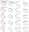
a, Scatterplots illustrating the noise levels of each estimated PC. Each plot shows population activity projected onto the specified principal component, for the 1st repeat (x-axis) and 2nd repeat (y-axis). Each point represents responses a a single stimulus. b, Estimated level of noise variance in successive signal dimensions. Noise variance was estimated by subtracting the cvPCA estimate of signal variance from the total variance (see Methods). c, Recovery of ground-truth eigenspectrum in simulated data. We simulated responses of 10,000 neurons to 2,800 stimuli with a power spectrum decay of exactly α = 1, and added noise in the stimulus space, generated with the spectrum in (b) scaled to produce the same signal-to-noise ratio as in the original neural data. The ground-truth eigenspectrum (black) is estimated accurately by the cvPCA method (blue). d, Same analysis with multiplicative noise, in which the responses of all neurons on each trial scaled by a common random factor. The distribution of this factor was again scaled to recover the original signal-to-noise ratio. e, Same analysis with a combination of multiplicative and additive noise. f, Same analysis, also including simulation of neural and 2-photon shot noise prior to running GCaMP deconvolution algorithm. g, 10 instantiations of the simulation were performed with ground-truth exponents of 0.5, 1.0, and 1.5. Error bars represent standard deviations of the power law exponents estimated for each of the 10 simulations. Dashed black line: ground-truth value. h-j, Comparison of cvPCA (yellow) and traditional PCA (green) algorithms in the presence of the additive+multiplicative noise combination. While cvPCA recovered the ground truth eigenspectrum (black) exactly, traditional PCA did not, resulting in overestimation of the top eigenvalues and failure to detect the ground-truth power law.

Extended Data Fig. 6. Successive PC dimensions encode finer stimulus features.

Each plot shows the responses of 10,145 neurons to 2,800 natural images, projected onto the specified PCs and then sorted along both axes so correlated neurons and stimuli are close together. We then smoothed the matrix across neurons and stimuli with Gaussian kernels of widths 8 neurons and 2 stimuli respectively. Dimensions 1-2 reveal a coarse, 1-dimensional organization of the neurons and stimuli. Dimensions 3-10 reveal multidimensional structure which involves different neural subpopulations responding to different stimuli. Dimensions 11-40 reveal finer-structured patterns of correlated selectivity among neurons. Dimensions 41-200 and 201-1000 reveal even finer-structured selectivity, which contained less neural variance.

Extended Data Fig. 7. Power law scaling reflects correlation structure, not single-neuron statistics.

a, The signal variance of each neuron’s responses are sorted in descending order; they approximately follow a power law with a decay exponent of α = 0.59. b, Same plot after z-scoring the recorded traces to equalize stimulus response sizes between cells; the distribution of single-neuron variance has become nearly flat. c PC eigenspectra for z-scored data. Each colored line represents a different recording. Dashed blue shows the average eigenspectrum from the original, non-z-scored responses. The fact that the eigenspectrum power-law is barely affected by equalizing firing rates, while the distribution of single cell signal variance is altered, indicates that the power law arises from correlations between cells rather than from the distribution of firing rates or signal variance across cells.

Extended Data Fig. 8. Power law eigenspectra in concatenated recordings.

a-c, To ask whether powerlaw eigenspectra apply to even larger populations, we were able to artificially double the number of recorded neurons by combining three pairs of recordings whose imaging fields of view had similar retinotopic locations. Top: retinotopic locations of receptive fields (95% confidence intervals on that recording’s mean RF position), with each recording shown in a different shade of blue. Bottom: eigenspectrum of concatenated recordings in response to the 2800 natural image stimuli; total population sizes 19571, 23472, and 18807 cells respectively. Each column represents one pair of recordings. d, Eigenspectrum exponents for random subsets of the combined populations (cf. Fig. 2j). X-axis shows population size relative to single recordings, so merged population is 2. Mean power law exponent at “2x” was α = 0.99 ± 0.02 (mean ± SE).

Extended Data Fig. 9. Eigenspectrum of electrophysiologically recorded data.

We recorded neural activity electrophysiologically in response to 700 out of the 2800 stimuli, and concatenated the recordings, resulting in a total of 877 neurons recorded across 6 experiments. a, With this smaller number of stimuli and neurons, convergence to a power law is not complete, and the exponent cannot be estimated accurately (cf. Fig. 2g-j). We therefore compared the electrophysiology data to a the responses generated by these stimuli in 877 neurons sampled randomly from either a single two-photon imaging experiment (dark blue) or all experiments combined (light blue). Red and pink show electrophysiology eigenspectra with time bins of 50 or 500ms; red line shows best linear fit to estimate exponent. b, Blue curves: power law exponents estimated from the responses of different-sized neuronal subpopulations to this set of 700 stimuli (shading: SE over different random subsets of neurons). Red and pink crosses: estimated exponsents from electrophysiology data for 50 and 500 ms bin sizes.

Extended Data Fig. 10. Power law scaling grows more accurate for increasing numbers of neurons and stimuli, for all stimulus ensembles.

a, Eigenspectra estimated from a random subset of the recorded neurons (color-coded by fraction of neurons retained. b, Eigenspectra estimated from a random subset of stimuli, color-coded by fraction of stimuli retained. c, Correlation coefficient of the spectra plotted in a,b. d, Power law exponent of the spectra plotted in a,b. Each row corresponds to a different ensemble of visual stimuli.

Figure 1. Population coding of visual stimuli.

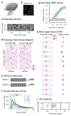
a, Simultaneous recording of ~10,000 neurons using 11-plane two-photon calcium imaging. b, Randomly-pseudocolored cells in an example imaging plane. c, Example stimulus spans three screens surrounding the mouse’s head. d, Mean responses of 65 randomly-chosen neurons to 32 image stimuli (96 repeats, z-scored, scale bar represents standard deviations, one recording out of four shown). e, A sequence of 2800 stimuli was repeated twice during the recording. f, Distribution of single-cell signal-to-noise ratios (SNR) (2800 stimuli, two repeats). Colors denote recordings; arrows represent means. g, Stimulus decoding accuracy as a function of neuron count for each recording. h, Example receptive fields (RFs) fit using reduced-rank regression or Gabor models (z-scored) (one recording shown, out of 7). i, Distribution of the receptive field centers, plotted on the left and center screens (line denotes screen boundary). Each cross represents a different recording, with 95% of neuron’s RF centers within error bars.

Figure 2. Visual cortical responses are high-dimensional with power-law eigenspectrum.

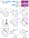
a, The eigenspectrum of visual stimulus responses was estimated by cross-validated principal component analysis (cvPCA), projecting singular vectors from the first repeat onto responses from the second. b, Cumulative fraction of variance in planes of increasing dimension, for an ensemble of 2800 stimuli (blue) and for 96 repeats of 32 stimuli. Dashed line indicates 32 dimensions. c, Eigenspectrum plotted in descending order of training set singular value for each dimension, averaged across 7 recordings (shaded error bars represent standard error). Black line denotes linear fit of 1/n^α. d Eigenspectra of each recording individually. e, Histogram of power law exponents α across all recordings. f, Cumulative eigenspectrum for a simple/complex Gabor model fit to the data (pink) superimposed on true data (blue). g, Eigenspectra computed from random subsets of recorded neurons, fraction indicated by colors. h, Same analysis for random subsets of stimuli. i, Pearson correlation of log variance and log dimension over dims 11-500, as a function of fraction analyzed (1 indicates a power law). j, Power law exponents of the spectra plotted in g,h.

Figure 3. Power law exponent depends on input dimensionality, but not image statistics.

a, Eigenspectra of natural image pixel intensities (gray), of visual cortical responses to these stimuli (blue), and of a simple/complex cell model’s response to these stimuli (pink). b, Same analysis for responses to spatially whitened stimuli, that lack 1/n image spectrum. c, Same analysis for images windowed over the RF of the recorded population. d, Same analysis for sparse noise stimuli. e, Same analysis for images projected into 8 dimensions produces a faster eigenspectrum decay with exponent α=1.49. f, After projecting images to 4 dimensions, α=1.65. g, Responses to drifting gratings, a one dimensional stimulus ensemble, show yet faster decay with α=3.43. h,i, Summary of power law exponents α for neural responses (h) and Gabor model (i), as a function of the dimensionality of the stimulus set d. Dashed line: α = 1 + 2/d, corresponding to the border of fractality.

Figure 4. The smoothness of simulated neural activity depends on the eigenspectrum decay.

Simulations of neuronal population responses to a 1-dimensional stimulus (x-axis), their eigenspectra, and a random projection of responses in 3D space. a, Wide tuning curves, corresponding to a circular neural manifold in a 2-dimensional plane. b, Narrow tuning curves corresponding to uncorrelated responses as predicted by the efficient coding hypothesis. c-e, Scale-free tuning curves corresponding to power law variance spectra, with exponents of 2, 3 (the critical value for d = 1), or 4. Tuning curves in c-e represent PC dimensions rather than individual simulated neurons.

References

1. Barlow HB. Possible principles underlying the transformations of sensory messages. In: Rosenblith W, editor. Sensory Communication. MIT Press; Cambridge, MA: 1961. pp. 217–234.
1. Atick JJ, Redlich AN. Towards a theory of early visual processing. Neural Computation. 1990;2:308–320.
1. Simoncelli EP, Olshausen BA. Natural image statistics and neural representation. Annual Review of Neuroscience. 2001;24:1193–1216. - PubMed
1. DiCarlo JJ, Zoccolan D, Rust NC. How does the brain solve visual object recognition? Neuron. 2012;73:415–434. - PMC - PubMed
1. Rigotti M, et al. The importance of mixed selectivity in complex cognitive tasks. Nature. 2013;497:585. - PMC - PubMed
Publication types