High-throughput profiling and analysis of plant responses over time to abiotic stress

Abstract

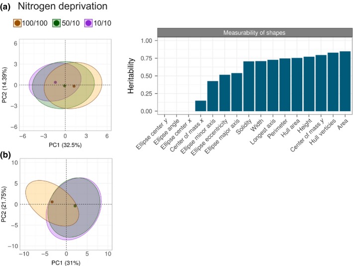
Sorghum (Sorghum bicolor (L.) Moench) is a rapidly growing, high-biomass crop prized for abiotic stress tolerance. However, measuring genotype-by-environment (G x E) interactions remains a progress bottleneck. We subjected a panel of 30 genetically diverse sorghum genotypes to a spectrum of nitrogen deprivation and measured responses using high-throughput phenotyping technology followed by ionomic profiling. Responses were quantified using shape (16 measurable outputs), color (hue and intensity), and ionome (18 elements). We measured the speed at which specific genotypes respond to environmental conditions, in terms of both biomass and color changes, and identified individual genotypes that perform most favorably. With this analysis, we present a novel approach to quantifying color-based stress indicators over time. Additionally, ionomic profiling was conducted as an independent, low-cost, and high-throughput option for characterizing G x E, identifying the elements most affected by either genotype or treatment and suggesting signaling that occurs in response to the environment. This entire dataset and associated scripts are made available through an open-access, user-friendly, web-based interface. In summary, this work provides analysis tools for visualizing and quantifying plant abiotic stress responses over time. These methods can be deployed as a time-efficient method of dissecting the genetic mechanisms used by sorghum to respond to the environment to accelerate crop improvement.

Keywords: abiotic stress; computational modeling; image analysis; ionomics; large‐scale biology; nitrogen stress.

Figure 1

Experimental Overview. (a) Watering regime used for nitrogen deprivation. The x‐axis shows the age of the plants throughout the experiment and the y‐axis indicates the estimated volume of water plus nutrients (ml), calculated based on the weight change of the pot before and after watering. Each dot represents the average amount of water delivered each day with vertical lines indicating error (99% confidence interval). Watering regime was increased due to plant age (shades of blue). The experimental treatments are listed above the plots. Volume of water and source of nitrogen are indicated and were scaled based on the 100% (100/100) treatment group (1 mm ammonium/14.5 mm nitrate for 100% treatment group). (b) Image analysis example (genotype NTJ2 from 100/100 treatment group on day 16 is shown). Top row: Example original RGB image taken from phenotyping system and plant isolation mask generated using PlantCV. Bottom row: two examples of attributes analyzed (area and color). Scale bar = 15 cm

Figure 2

Determining plant attributes affected by experimental treatments. (a) Left: Principal component analysis (PCA) plots of shape attributes for plants subjected to nitrogen deprivation at the end of the experiment (plant age 26 days). 95% confidence ellipses are calculated for each of the treatment groups and the dots indicate the center of mass. The shape attributes included in the PCA are as follows: area, hull area, solidity, perimeter, width, height, longest axis, center of mass x‐axis, center of mass y‐axis, hull vertices, ellipse center x‐axis, ellipse center y‐axis, ellipse major axis, ellipse minor axis, ellipse angle, and ellipse eccentricity. Right: Bar graph indicating measurability of shape attributes, showing the proportion of variance explained by treatment (i.e., treatment effect, y‐axis). (b) PCA plots showing analysis of color values within the mask for plants subjected to nitrogen deprivation at the end of the experiment (plant age 26 days). All 360 degrees of the color wheel were included, binned every 2 degrees

Figure 3

Growth response of genotypes to nitrogen deprivation. (a) Box plot showing average plant size (area) at the end of the experiment (day 26), * q‐values < 0.01) with outliers (dots) at the end of the experiment for the 10/10 treatment group. The median is indicated by a black bar within each box. (b) Growth rate (average change in area per day, days 10–22) for the 10/10 treatment group. The dotted lines indicate the treatment group average in both panels. Genotypes that displayed greater than average (blue) or less than average (magenta) growth are indicated. Error bars: 95% confidence intervals for both graphs

Figure 4

Timing of response to nitrogen: size changes in late‐ and early‐responding genotypes. (a) Statistical analysis of differences in area over time (bottom, plant age) for the 30 sorghum genotypes analyzed. q‐values for the heat map are indicated in blue, with darkest coloring representing most significance. The Canberra distance‐based cluster dendrogram (right) was generated from calculated q‐values. (b) Box plots showing average biomass (area) with outliers (colored dots) for late (left)‐ and early (right)‐responding lines from panel A at the beginning (day 8, top) and end (day 26, bottom) of the experiment. The median is indicated by a black bar within each box. * indicates significant difference between early and late groups (p‐value < 5 × 10⁻⁶). (c) Scatter plots representing plant area (y‐axis) by treatment (x‐axis) at the beginning (day 8), middle (day 19), and end (day 26) of the experiment for chosen late‐responding (left) and early‐responding (right) genotypes (key, right). Each dot represents an individual plant on a day and dotted lines connect genotypic averages

Figure 5

Color changes in late‐ and early‐responding genotypes to nitrogen treatment. (a) Average histograms illustrating percentage of identified plant image mask (y‐axis) represented by a particular hue degree (x‐axis). Presented is the average of the early‐ and late‐responding lines on day 13 of the experiment. Yellow and green areas of the hue spectrum are highlighted as such. (b) Change in yellow (degrees 0–60) and green (degrees 61–120) hues over time for 100/100 (left) and 10/10 (right) treatment groups. Plotted is the area under the curves presented in A (y‐axis) over the duration of the experiment (x‐axis) for early‐ and late‐responding genotypes. Gray areas indicate standard error

Figure 6

Ionomic profiling of genotypes at the end of the experiment. (a) The percent variance explained by each partition of the total variance model (above). (b) Left: PCA plots (all elements) colored by treatment for individual genotypes (left) and 95% confidence ellipses (right). The percent variance explained by each component is indicated in parentheses. Right: loadings for each element from the first two PCs are shown on the y‐axis and are color filled based on the direction and strength of the contribution. Positive direction is colored blue and negative direction is colored red. For a given element, the color for PC1 and PC2 is related by the unit circle and saturation of the color is equal to the length of the projection into each of the two directions. (c) Boxplots representing dry weight concentrations for all elements and all nitrogen treatments. Concentrations are reported as parts per million (y‐axis: mg analyte/kg sample) for each genotype (x‐axis). The median is indicated by a black bar within each box. Magenta line: mean phosphorus concentration for given treatment group