Quantitative phase imaging of adherent mammalian cells: a comparative study

Abstract

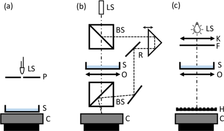
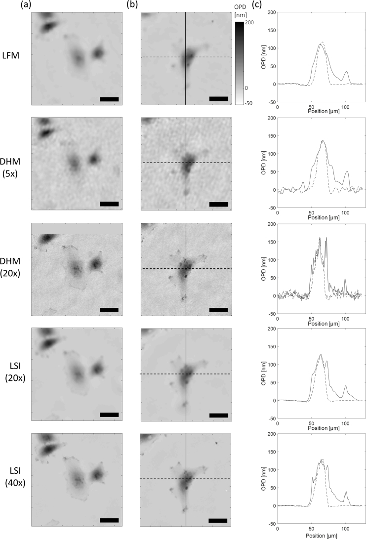
The Quantitative phase imaging methods have several advantages when it comes to monitoring cultures of adherent mammalian cells. Because of low photo-toxicity and no need for staining, we can follow cells in a minimally invasive way over a long period of time. The ability to measure the optical path difference in a quantitative manner allows the measurement of the cell dry mass, an important metric for studying the growth kinetics of mammalian cells. Here we present and compare cell measurements obtained with three different techniques: digital holographic microscopy, lens-free microscopy and quadriwave lateral sheering interferometry. We report a linear relationship between optical volume density values measured with these different techniques and estimate the precisions of this measurement for the different individual instruments.

Fig. 1

Optical setups a) LFM b) DHM c) LSI. LS light source, P pinhole, S sample, C camera, O microscope objective, BS beam splitter, R variable length reference arm, K Kohler illumination system, F band-pass filter, H modified Hartmann mask. Note that light source is partially coherent for LSI (Kohler illumination), and LFM (LED with a pinhole) and coherent (laser) for DHM (b). Modified Hartmann mask H and camera C in (c) compose the Phasics camera mounted on a standard wide-field microscope.

Fig. 2

(a, b) OPD maps of the same fixed COS-7 cells obtained with the different techniques. Scale bar is 25 μm. (c) OPD profiles measured through the cell center in (b) (solid line: vertical, dashed line: horizontal).

Fig. 3

Subtraction of the baseline image. (a) OPD raw map of a COS-7 cell (fixed) obtained by LSI(40×). (b) Estimation of the baseline image. (c) Final result after baseline subtraction, i.e. image(a)-image(b). Scale bar is 25 μm. (d, e, f) OPD profiles measured in the images (a, b, c) through the cell center (solid line: vertical, dashed line: horizontal). (g) The results of the baseline subtraction algorithm (black dots) are given by spatial variation measurements of the OPD values in sample-free area of 50×50 μm². The different points correspond to different parameters used in the baseline subtraction algorithm. One black dot depicts the average value over several tens of OPD map. The measurements before baseline subtraction are plotted with red crosses.

Fig. 4

Comparison between LSI(40×) and LFM. (a) OPD map of a fixed COS-7 cell obtained with LSI(40×). Scale bar is 25 μm. The contour of the ground truth cell segmentation area is shown in black. (b) OPD map obtained with LFM. (c) Pixel to pixel comparison between the OPD maps (within segmented cell area). The results of the linear regressions are indicated with values of slope, intercept, coefficient of determination (R²) and root-mean-square deviation (RMSD). (d) OVD obtained with LFM when introducing registration errors of ±1 μm on the X–Y position and ±0.5 degree on the rotation. The results are shown with and without the use of the best-matching algorithm, which counterbalances these errors. (e) Plot of the cell OVD measurements for different baseline subtraction algorithm parameters.

Fig. 5

Pair-wise comparisons of OVD measurements of fixed COS-7 cells. The OVD measurements are obtained with the ground truth cell segmentation and the baseline subtraction algorithm parameters which minimize the spatial variation in the sample-free area. The linear regression fitting curves are plotted in black. The results of the linear regressions are indicated with values of slope, intercept, coefficient of determination (R²) and root-mean-square deviation (RMSD). N refers to the number of cell OVD measurements per comparison.

Fig. 6

(a, b, c) OPD image of fixed COS-7 cells obtained with (a) LFM, (b) DHM(20×) and (c) LSI(40×). The 9 cells of interest are numbered. (d, e, f) OVD measured on the 9 cells of interest over 50 consecutive acquisitions with LFM, DHM(20×) and LSI(40×).

Fig. 7

Estimations of the instrument precisions. (a) Results obtained with manual ground truth cell segmentation. The different point correspond to different parameters used in the baseline subtraction algorithm, i.e. the sensitivity of the adaptive thresholding filter (ranging from 0.5 to 1), two different OPD threshold values (ranging from 2.5 nm to 12.5 nm) and the order of the polynomial fitting of the OPD values in sample-free area (ranging from 3 to 10). The red crosses point out the results obtained with the baseline subtraction algorithm which minimizes the spatial variation in the sample-free area (see Fig. 3). The results of the optimized baseline subtraction algorithm are shown with red circles (see appendix A.2). (b) Results obtained with automatic cell segmentation. The different points correspond to different threshold values used in the seeded growing segmentation algorithm ranging between 5 nm and 17.5 nm. The red circles correspond to the results obtained with threshold values of 10 nm for LFM, 12.5 nm for DHM and 5 nm for LSI.

Fig. 8

(a–c) Automatic seeded growing segmentation of a fixed COS-7 cell as a function of the threshold parameter value. The contour of the automatic segmentation and the manual ground truth are overlaid in orange and black, respectively. (d) Plot of the mean IoU (intersection over union) value and the mean ratio between the OVD measurements obtained with the automatic segmentation (OVD_SEG) and the ground truth manual cell segmentation (OVD_GT) as a function of the segmentation threshold value for the different modalities.