The community structure of functional brain networks exhibits scale-specific patterns of inter- and intra-subject variability

Abstract

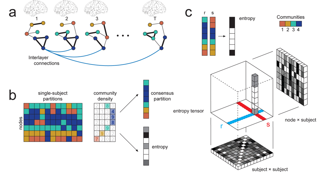
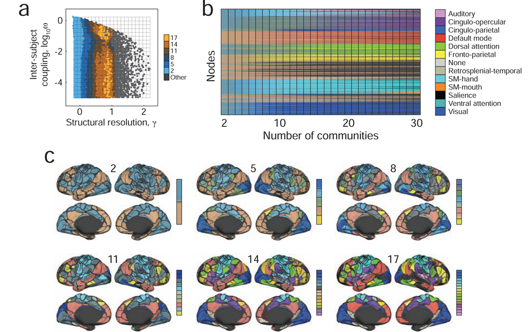
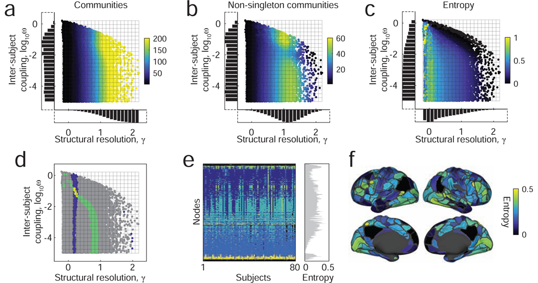
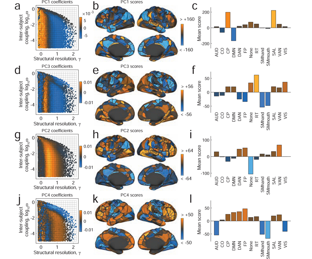
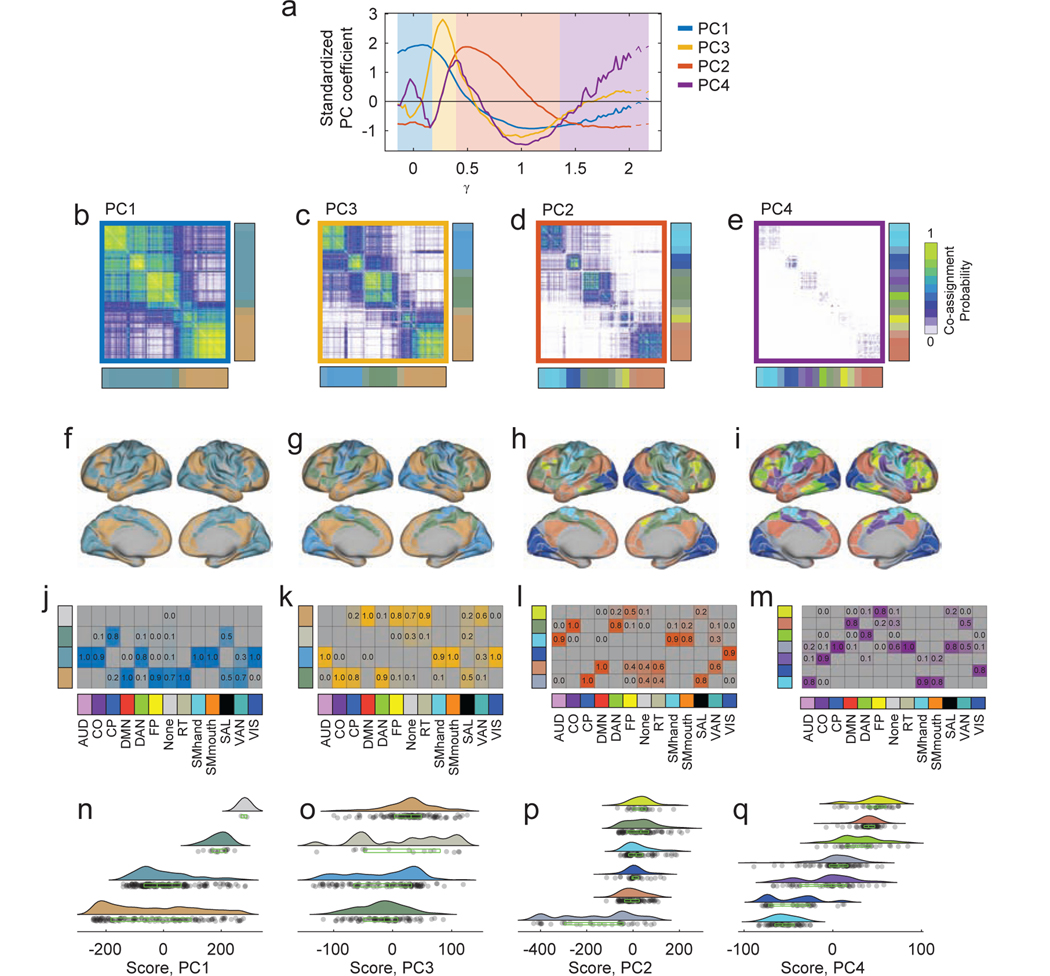
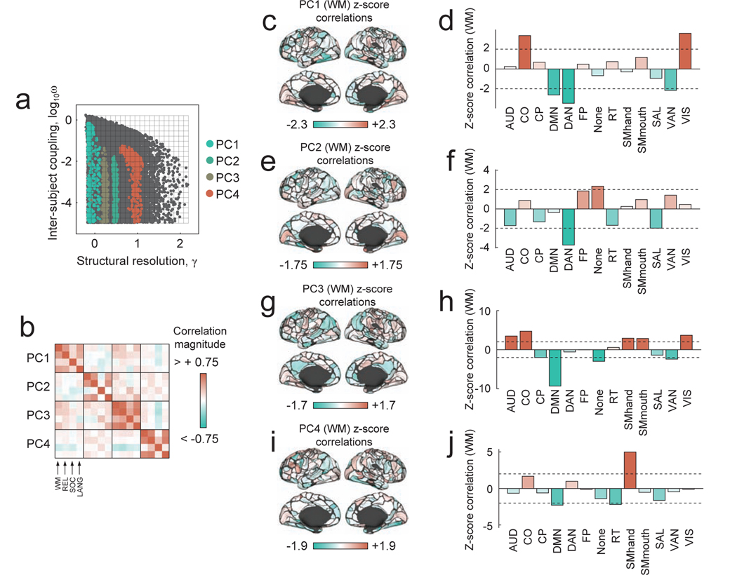
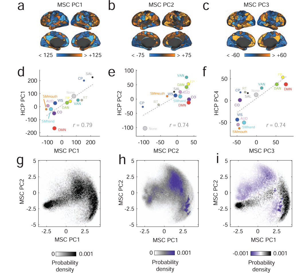
The network organization of the human brain varies across individuals, changes with development and aging, and differs in disease. Discovering the major dimensions along which this variability is displayed remains a central goal of both neuroscience and clinical medicine. Such efforts can be usefully framed within the context of the brain's modular network organization, which can be assessed quantitatively using computational techniques and extended for the purposes of multi-scale analysis, dimensionality reduction, and biomarker generation. Although the concept of modularity and its utility in describing brain network organization is clear, principled methods for comparing multi-scale communities across individuals and time are surprisingly lacking. Here, we present a method that uses multi-layer networks to simultaneously discover the modular structure of many subjects at once. This method builds upon the well-known multi-layer modularity maximization technique, and provides a viable and principled tool for studying differences in network communities across individuals and within individuals across time. We test this method on two datasets and identify consistent patterns of inter-subject community variability, demonstrating that this variability - which would be undetectable using past approaches - is associated with measures of cognitive performance. In general, the multi-layer, multi-subject framework proposed here represents an advance over current approaches by straighforwardly mapping community assignments across subjects and holds promise for future investigations of inter-subject community variation in clinical populations or as a result of task constraints.

FIG. 1.. Multi-subject modularity, communities, and areal entropy.

(a) Single-subject networks are represented as layers in a multi-layer network ensemble. Each node is linked to itself across layers, here illustrated by interlayer connections. Note that community labels are indicated by node color. (b) Maximizing a multi-layer modularity function returns a set of single-subject partitions. Importantly, community labels are preserved across layers; thus, if the label C₁ appears in layers r and s, we assume that the same community has recurred. This property allows us to make several useful measurements. We can calculate, for each node, the mode of its community assignment across subjects to generate a consensus partition. We can also calculate the entropy of each node’s community assignments, which measures the variability of communities across subjects. (c) The preservation of community labels also allows for a direct comparison of any one subject to any other subject. Given partitions of subjects (or layers), denoted here with variables r and s, we can generate a bit vector whose values are {0, 1} depending on whether a given node has the same/different community assignment. Doing so for all pairs of subjects generates a three-dimensional entropy tensor. When averaged over nodes, this tensor generates a T ×T matrix whose elements indicate, in total, the number of non-identical community assignments between pairs of subjects. When averaged over either of its other dimensions, the result is an N × T matrix, whose elements indicate, in total, the similarity of a node’s community assignment within a given subject to that of the remaining T − 1 subjects.

FIG. 2.. Examples of detected community structure.

(a) The composition of detected communities depends on the structural resolution parameter, γ, and on the inter-subject coupling parameter, ω. To generate a sample of possible partitions, we chose random combinations of γ and ω and estimate consensus community structure at those points. We show, here, the locations in parameter space where the resulting consensus partitions contained 2, 5, 8, 11, 14, and 17 non-singleton communities per subject. (b) We ordered all consensus partitions in ascending order according to their number of non-singleton communities. Each community was colored by the weighted average of its constituent brain areas’ cognitive systems. For example, a community comprised of exclusively DMN brain areas would be assigned the DMN color (red, in this case), whereas a system composed of an equal number of DMN and visual brain areas would have a purple color (the average of the DMN’s red and the visual system’s blue). (c) We also show example consensus partitions as we vary the number of non-singleton communities to 2, 5, 8, 11, 14, and 17.

FIG. 3.. Multi-scale analysis strategy and schematic.

Points are sampled in a two-dimensional constrained parameter space. The structural resolution parameter, γ, determines the number and size of communities while the inter-layer coupling parameter, ω, tunes the consistency of communities across individuals. Here, we summarize the statistics of communities detected using this sampling approach applied to the HCP333 dataset. (a) The number of communities per layer. (b) The number of communities per layer after excluding singleton communities, which are communities composed of a single node. (c) The mean inter-subject entropy (variability). (d) We can query particular subsets of partitions based on the number of communities, their average entropy, or other statistics, allowing us not only to probe different organizational scales of the network, but also to accommodate varying degrees of heterogeneity across subjects. (e) An example of the detected partitions and their consistency across T = 80 subjects. (f) The variability (inter-subject entropy) of community assignments across individuals. Brighter (yellow) coloring indicates greater levels of variability.

FIG. 4.. Modes of inter-subject community variability.

Principal component coefficients and scores for the first four components. (a) PC coefficients for the first component projected into {γ, ω} parameter space. (b) PC scores for the same component projected onto the cortical surface. The community assignments of bright orange brain areas are highly variable across subjects at orange points in the parameter space. Conversely, the community assignments of blue brain areas are highly consistent across subjects at those same points. (c) Areal values of principal component scores averaged across thirteen previously-defined cognitive/functional systems [26]. This panel helps shift focus away area-level community variability and onto system level patterns of variation. The remaining panels show corresponding plots for PC₂, PC₃, and PC₄. Note: we present principal components in the order in which they are expressed along the γ axis. This choice results in the following ordering: PC₁, PC₃, PC₂, and PC₄.

FIG. 5.. Community structure changes as a function of γ.

We restricted our analysis to the region of parameter space with ω < 10⁻². Within this space, virtually all variation in community structure occurs as a function of γ. We then calculated the average PC coefficient for each of the four PCs as a function of γ and z-scored these values for each PC independently. (a) This procedure enabled us to partition γ values into four segments according to which PC is dominant at that point in parameter space. (b-e) For each segment, which corresponded to a different PC’s dominance, we calculated the co-assignment probability for all pairs of nodes. (f - i) We also derived each segments’ consensus communities. (j-m) We also assessed how brain systems described in [26] are distributed across detected communities. In these panels, each column corresponds to one of the thirteen systems and each row corresponds to a detected community. Columns were normalized so that they sum to unity. Within a column the values of cells indicate the fraction of that system’s regions that were assigned to each of the detected communities. (n-q) We break down the PC scores by detected communities.

FIG. 6.. Correlation of community structure with measures of task performance.

(a) For each PC, we studied the sub-sample of partitions corresponding to the 1% largest PC coefficients. (b) For each subsample, we calculated the Pearson correlation coefficient between subjects’ community entropy scores and four measures of in-scanner performance on cognitively demanding tasks: working memory (WM), relational (REL), social (SOC), and language (LANG), in the HCP terminology. In panels (c,e,g,i), we show the brain-behavior z-scored correlation coefficients for the first four PCs associated with performance on the WM task, plotted on the cortical surface (permutation test in which behavioral measures were randomly and uniformly shuffled). In panels (d,f,h,j), we show the mean brain-behavior correlation coefficients for the first four PCs, z-scored within each cognitive system. Larger z-scores indicate that the average correlation over all brain areas in a given system is greater than expected in random systems of the same size. Here, as an example, we show correlations for the WM task. Results for other tasks are included in the Supplementary Materials. Note that the dotted lines in panels (d), (f), (h), and (j) correspond to z = ±2.

FIG. 7.. Summary and analysis of the midnight scan club dataset.

In panels (a)-(c), we show surface maps depicting the first three components generated from PCA analysis of the midnight scan club (MSC) dataset. These principal components correspond, broadly, to the components detected in the HCP dataset. We compare the two datasets by averaging principal components within brain systems and computing system-average correlations. The results are shown in panels (d)-(f). The size of dots is proportional to the number of nodes assigned to each system. We perform a similar analysis of intra-subject variability, in which we characterize variation in community structure within subjects across scan sessions. To visualize these results, we project within- and between-subject community entropy scores into the two-dimensional space defined using the first two dimensions of a joint PCA. In panel g, we show the distribution of inter-subject patterns. Panel h shows the same for intra-subject patterns, and i shows the difference between the two.

References

1. Bullmore Ed and Sporns Olaf, “Complex brain networks: graph theoretical analysis of structural and functional systems,” Nature Reviews Neuroscience 10, 186 (2009). - PubMed
1. Betzel Richard F and Bassett Danielle S, “Multi-scale brain networks,” Neuroimage 160, 73–83 (2017). - PMC - PubMed
1. Newman Mark EJ, “Communities, modules and large-scale structure in networks,” Nature physics 8, 25 (2012).
1. Sporns Olaf and Betzel Richard F, “Modular brain networks,” Annual review of psychology 67, 613–640 (2016). - PMC - PubMed
1. Power Jonathan D, Cohen Alexander L, Nelson Steven M, Wig Gagan S, Barnes Kelly Anne, Church Jessica A, Vogel Alecia C, Laumann Timothy O, Miezin Fran M, Schlaggar Bradley L, et al. , “Functional network organization of the human brain,” Neuron 72, 665–678 (2011). - PMC - PubMed
Publication types