Mathematical modelling for sustainable aphid control in agriculture via intercropping

Abstract

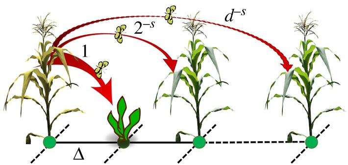
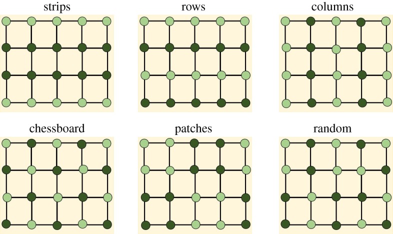
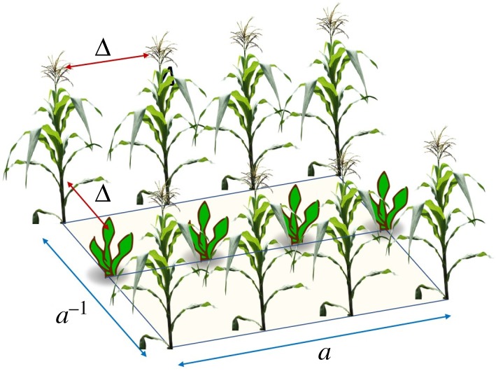
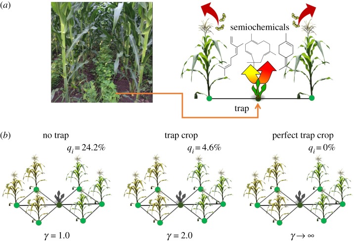
Agricultural losses to pests represent an important challenge in a global warming scenario. Intercropping is an alternative farming practice that promotes pest control without the use of chemical pesticides. Here, we develop a mathematical model to study epidemic spreading and control in intercropped agricultural fields as a sustainable pest management tool for agriculture. The model combines the movement of aphids transmitting a virus in an agricultural field, the spatial distribution of plants in the intercropped field and the presence of 'trap crops' in an epidemiological susceptible-infected-removed model. Using this model, we study several intercropping arrangements without and with trap crops and find a new intercropping arrangement that may improve significantly pest management in agricultural fields with respect to the commonly used intercrop systems.

Keywords: agriculture; aphid-borne virus transmission; complex networks; intercropping; plant infections; trap crops.

Figure 1.

Inter-plants movements of an aphid in an agricultural plot with intercropping (see electronic supplementary material, Note 1). The hop of an aphid from an infected plant to a susceptible one separated by d steps is given by d^−s (see electronic supplementary material, Notes 1 and 2). (Online version in colour.)

Figure 2.

Intercrop arrangements. Different organizations of intercrops between two species studied in this work with r = Δ (see Network construction). Light green nodes represent the main crop and dark green nodes represent the secondary crop, which is considered to be not susceptible to the disease spreading on the field. In the case of trap crop strategies, the dark green nodes represent the plants with semiochemical activity to trap the pest to be controlled. The square lattices connecting the nodes correspond to the interconnection networks considered here. (Online version in colour.)

Figure 3.

Schematic of the intercropping of two species in a rectangular plot of unit area and largest edge length a. The separation between plants is given by Δ. (Online version in colour.)

Figure 4.

(a) Intercropping with ‘push’ (or push–pull) strategies where semiochemicals [72,73] are released from trap crops (photograph courtesy of Rachel Monger (Immanuel International)). (b) Effects of the strength of the trap crop γ (small dark plants) on the probability of plants i becoming infected q_i (see text for explanations) once the plants on the left of the figures are infected. (Online version in colour.)

Figure 5.

Evolution of the number of infected plants in a square plot with varying time delays τ. The modelling is performed with β = 0.5, μ = 0.5, r = Δ and s = 2.5 (a) and s = 1.0 (b). (Online version in colour.)

Figure 6.

Aphid-borne virus propagation on intercropped fields without traps. Results of the simulations for SIR epidemics at t = 10 with r = Δ, β = 0.5, μ = 0.5 for different intercropping strategies without trap crops, i.e. the strength of the trap crop is γ = 1.0. Raincloud plots of the proportion of dead plants for a viral infection propagated by aphids: (a) aphid with reduced mobility (s = 4.0) and (b) with greater mobility (s = 2.5). The clouds show the kernel distribution of the proportion of dead plants for different realizations of the epidemics. Below, the raw data are plotted (the rain) together with their corresponding box and whisker plots. Illustration of the evolution of infection across fields with different intercropping systems: (c) aphid with reduced mobility (s = 4.0) and (d) with greater mobility (s = 2.5). In both panels, the time t* is given in a colour scale (see text), and the propagation is initialized by infecting the plant in the bottom-left corner of the plot. (Online version in colour.)

Figure 7.

Aphid-borne virus propagation on intercropped fields with trap crops. Results of the simulations for SIR epidemics at t = 10 with r = Δ, β = 0.5, μ = 0.5 for different intercropping strategies with trap crops of strength γ = 2.0. Raincloud plots of the proportion of dead plants for a viral infection propagated by aphids: (a) aphid with reduced mobility (s = 4.0) and (b) with greater mobility (s = 2.5). The clouds show the kernel distribution of the proportion of dead plants for different realizations of the epidemics. Below, the raw data are plotted (the rain) together with their corresponding box and whisker plots. Illustration of the evolution of infection across fields with different intercropping systems: (c) aphid with reduced mobility (s = 4.0) and (d) with greater mobility (s = 2.5). In both panels, the time t* is given in a colour scale (see text), and the propagation is initialized by infecting the plant in the bottom-left corner of the plot. (Online version in colour.)

Figure 8.

Epidemic thresholds for the propagation of aphid-borne viruses on intercropped fields. Effects of the strength of the trap crop γ and of the pest mobility s on the number of removed (dead) plants during the propagation of an aphid-borne virus infection across intercropped fields with r = Δ. The case for γ = 1 corresponds to no trap crop. The symbols used for each intercrop are: strips (small circles), rows (large circles), columns (squares), chessboard (triangles), patches (hexagons), random (diamonds) and monocrop (crosses). In the insets, we illustrate the normalized epidemic thresholds for each of the intercrop arrangements. The normalization is obtained by dividing every epidemic threshold by that of the monocrop in the corresponding system. The colour code for the insets is given at the bottom of the figure. In each inset, the columns are ordered as the labels of the legend. (Online version in colour.)