Best fitting tumor growth models of the von Bertalanffy-PütterType

Abstract

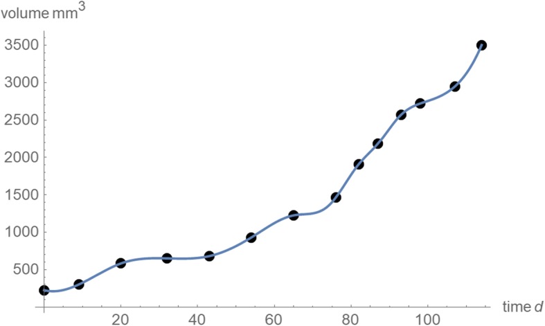
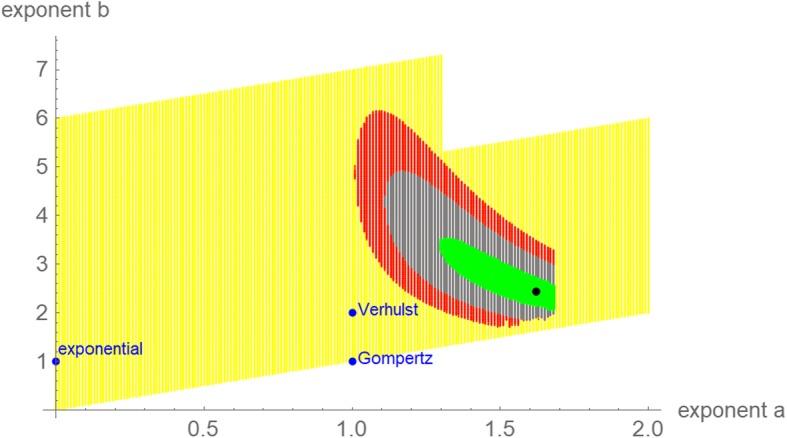
Background: Longitudinal studies of tumor volume have used certain named mathematical growth models. The Bertalanffy-Pütter differential equation unifies them: It uses five parameters, amongst them two exponents related to tumor metabolism and morphology. Each exponent-pair defines a unique three-parameter model of the Bertalanffy-Pütter type, and the above-mentioned named models correspond to specific exponent-pairs. Amongst these models we seek the best fitting one.

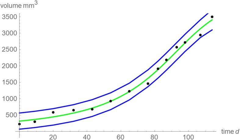
Method: The best fitting model curve within the Bertalanffy-Pütter class minimizes the sum of squared errors (SSE). We investigate also near-optimal model curves; their SSE is at most a certain percentage (e.g. 1%) larger than the minimal SSE. Models with near-optimal curves are visualized by the region of their near-optimal exponent pairs. While there is barely a visible difference concerning the goodness of fit between the best fitting and the near-optimal model curves, there are differences in the prognosis, whence the near-optimal models are used to assess the uncertainty of extrapolation.

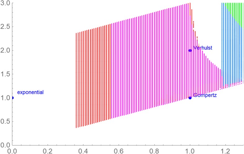
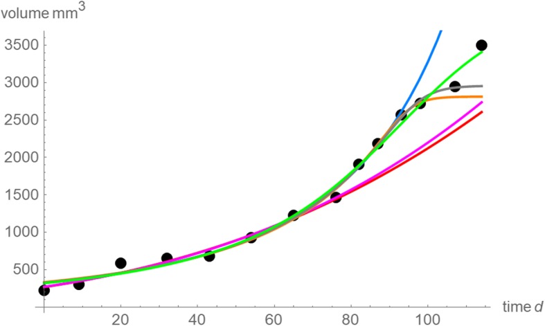
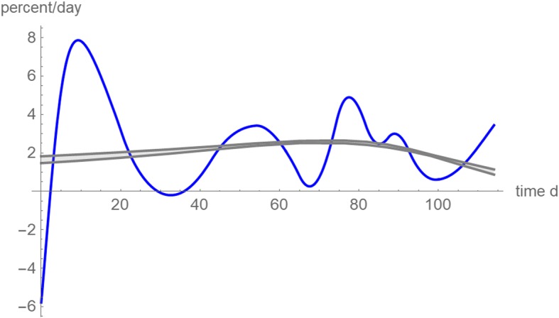
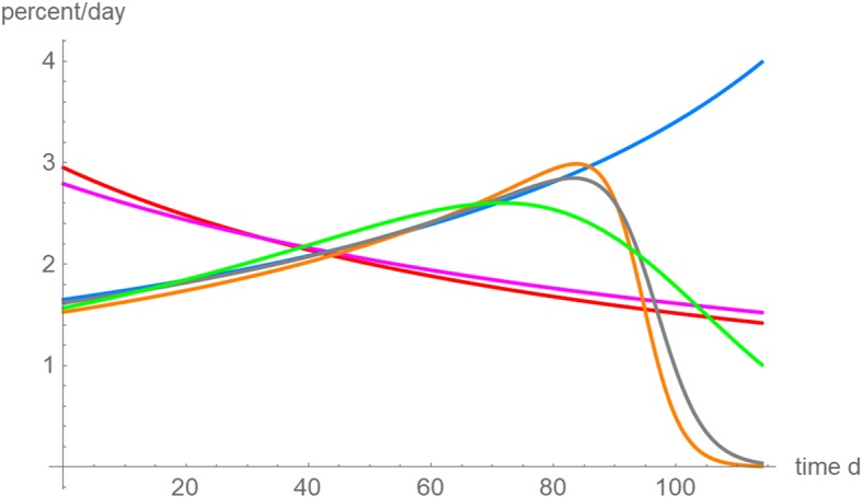
Results: For data about the growth of an untreated tumor we found the best fitting growth model which reduced SSE by about 30% compared to the hitherto best fit. In order to analyze the uncertainty of prognosis, we repeated the search for the optimal and near-optimal exponent-pairs for the initial segments of the data (meaning the subset of the data for the first n days) and compared the prognosis based on these models with the actual data (i.e. the data for the remaining days). The optimal exponent-pairs and the regions of near-optimal exponent-pairs depended on how many data-points were used. Further, the regions of near-optimal exponent-pairs were larger for the first initial segments, where fewer data were used.

Conclusion: While for each near optimal exponent-pair its best fitting model curve remained close to the fitted data points, the prognosis using these model curves differed widely for the remaining data, whence e.g. the best fitting model for the first 65 days of growth was not capable to inform about tumor size for the remaining 49 days. For the present data, prognosis appeared to be feasible for a time span of ten days, at most.

Keywords: Bertalanffy-Pütter growth models; Cancer; Simulated annealing; Tumor growth.

Fig. 1

Exponent-pairs of well-known named models (blue dots and grey lines); exponent-pairs that were considered in an initial search for the best fitting model (yellow)

Fig. 2

Size-at-age data (black dots) from Table 1 and cubic splines (blue). Additional statistical information (e.g. standard deviations) was not available for the original data

Fig. 3

Extended search grid (yellow) with 106,599 grid-points; selected exponent-pairs (blue); optimal exponent-pair (black) a = 1.62, b = 2.44 for the fit to the growth data over 114 days; 17,403 and 9,416 and 2,315 near-optimal exponent-pairs (red, gray, and green) for the thresholds 10, 5, and 1%, respectively (i.e. for the exponent-pairs SSE_opt exceeded the minimal SSE by at most that threshold). The optimal parameters obtained from simulated annealing are displayed in Table 2. The parameters were slightly improved in Fig. 4

Fig. 4

Data (black dots); single prediction band (95% confidence: blue); best fitting model curve (green): optimal exponent-pair a = 1.62, b = 2.44 and (slightly improved) parameters v₀ = 317.9 mm³ (95%-confidence limits, 249.2 to 386.5), p = 5·10^− 4 (4·10^− 4 to 6.1·10^− 4) and q = 5.6·10^− 7 (3.7·10^− 7 to 7.4·10^− 7)

Fig. 5

Optimal exponent-pairs for different data, labeled by their time spans of observation. The yellow line is the lower bound for the exponent-pair region (diagonal a = b)

Fig. 6

Regions of near-optimal exponent-pairs within the search grid of Fig. 1 for four data, whose SSE_opt did not exceed the minimal SSE for the respective data by more than 5%: data for 65 days (red, violet and the lower part of blue); for 76 days (violet and the lower part of blue); for 87 days (blue and green); and for 114 days (green). The regions for 98 and 107 days were outside the considered search grid. The exponent-pairs of three named models were displayed for better orientation (dark blue)

Fig. 7

Search grid (yellow), optimal exponent-pair (black) for finding the best fitting model curve to the data of the first 107 days of tumor growth, and near-optimal exponent pairs (red), using a threshold of 5%

Fig. 8

Model curves (exponents and parameters in Table 2) with the best fit to the following data (black dots): data for 65 days (red); data for 76 days (violet); data for 87 days (blue); data for 98 days (orange), data for 107 days (gray) and data for 114 days (green)

Fig. 9

Relative growth rates (percent/day) of the best fitting model curves from 2,315 near-optimal exponent-pairs (their SSE_opt exceeds the minimal SSE by at most 1%). The shaded area is the region between the minimal and maximal growth rates that some model reached at that day. The blue curve is the relative growth rate computed from the spline interpolation function of Fig. 2 (a method for the numeric differentiation of the data)

Fig. 10

Relative growth rates (percent/day) based on the best fitting model curves for different data: data for 65 days (red); data for 76 days (violet); data for 87 days (blue); data for 98 days (orange), data for 107 days (gray) and data for 114 days (green)

References

1. Schwartz M. A biomathematical approach to clinical tumor growth. Cancer. 1961;14:1272–1294. doi: 10.1002/1097-0142(196111/12)14:6<1272::AID-CNCR2820140618>3.0.CO;2-H. - DOI - PubMed
1. Bloom HJ, Richardson WW, Harries EJ. Natural history of untreated breast cancer. Comparison of untreated and treated cases according to histological grade of malignancy. Br Med J. 1962;2:213–221. doi: 10.1136/bmj.2.5299.213. - DOI - PMC - PubMed
1. Laird AK. Dynamics of tumor growth. Br J Cancer. 1965;19:278–291. doi: 10.1038/bjc.1965.32. - DOI - PMC - PubMed
1. Wheldon, T.E. Mathematical models in Cancer research, Bristol (UK): Adam Hilger1988.
1. Michor F. Evolutionary dynamics of cancer. Doctoral thesis. Cambridge: Harvard Univ; 2005.
LinkOut - more resources