Evaluation of Deep Learning Strategies for Nucleus Segmentation in Fluorescence Images

Abstract

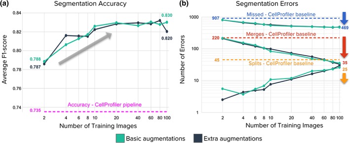
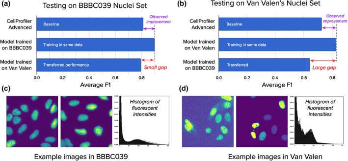
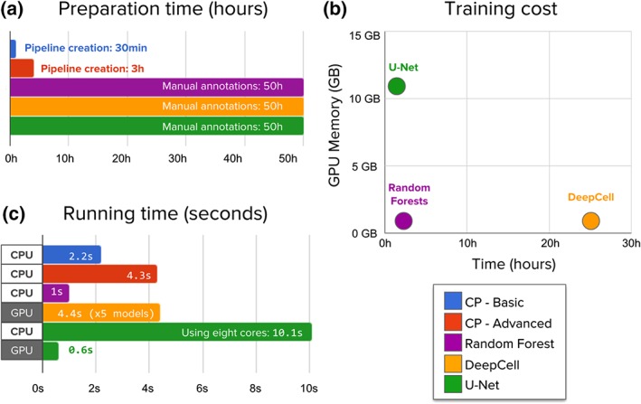
Identifying nuclei is often a critical first step in analyzing microscopy images of cells and classical image processing algorithms are most commonly used for this task. Recent developments in deep learning can yield superior accuracy, but typical evaluation metrics for nucleus segmentation do not satisfactorily capture error modes that are relevant in cellular images. We present an evaluation framework to measure accuracy, types of errors, and computational efficiency; and use it to compare deep learning strategies and classical approaches. We publicly release a set of 23,165 manually annotated nuclei and source code to reproduce experiments and run the proposed evaluation methodology. Our evaluation framework shows that deep learning improves accuracy and can reduce the number of biologically relevant errors by half. © 2019 The Authors. Cytometry Part A published by Wiley Periodicals, Inc. on behalf of International Society for Advancement of Cytometry.

Keywords: chemical screen; deep learning; fluorescence imaging; image analysis; nuclear segmentation.

Figure 1

Strategy of the evaluated deep learning approaches. Our main goal is to follow the popular strategy of segmenting each nucleus and micronucleus as a distinct entity, regardless of whether it shares the same cell body with another nucleus. It is generally possible to group nuclei within a single cell using other channels of information in a postprocessing step if the assay requires it. (a) Images of the DNA channel are manually annotated, labeling each nucleus as a separate object. Then, labeled instances are transformed to masks for background, nucleus interior, and boundaries. A convolutional neural network (CNN) is trained using the images and their corresponding masks. (b) The trained CNN generates predictions for the three class classification problem. Each pixel belongs to only one of the three categories. In postprocessing, the predicted boundary mask is used to identify each individual instance of a nucleus. [Color figure can be viewed at wileyonlinelibrary.com]

Figure 2

Segmentation performance of five strategies compared against ground‐truth expert segmentations. (a) Average F ₁‐score versus nucleus coverage for U‐Net (green), DeepCell (yellow), Random Forest (purple), CellProfiler advanced (red), and CellProfiler basic (blue). The y axis is average F ₁‐score (higher is better), which measures the proportion of correctly segmented objects. The x axis represents intersection‐over‐union (IoU) thresholds as a measurement of how well aligned the ground truth and estimated segmentations must be to count a correctly detected nucleus. Higher thresholds indicate stricter boundary matching. Notice that average F ₁‐scores remain nearly constant up to IoU = 0.80; at higher thresholds, performance decreases sharply, which indicates that the proportion of correctly segmented objects decreases when stricter boundaries are required to count a positive detection. (b) Example segmentations obtained with each of the five evaluated methods sampled to illustrate performance differences. Segmentation boundaries are in red, and errors are indicated with yellow arrows. [Color figure can be viewed at wileyonlinelibrary.com]

Figure 3

Analysis of segmentation errors (missed and extra objects). The 5,720 nuclei in the test set were used in this analysis. (a) Fraction of missed nuclei by object size (see table). Missed objects in this analysis were counted using an IoU threshold of 0.7, which offers a good balance between strict nucleus coverage and robustness to noise in ground truth annotations. (b) Example image illustrating sizes of nuclei. (c) Fraction of extra or false objects introduced by algorithms. [Color figure can be viewed at wileyonlinelibrary.com]

Figure 4

Analysis of segmentation errors (splits and merged objects). The 5,720 nuclei in the test set were used in this analysis. (a) Fraction of merged and split nuclei. These errors are identified by masks that cover multiple objects with at least 0.1 IoU. (b) Example merges and splits. [Color figure can be viewed at wileyonlinelibrary.com]

Figure 5

Impact of the number of annotated images used for training a U‐Net model. Basic augmentations include flips, 90° rotations, and random crops. Extra augmentations include the basic plus elastic deformations. (a) Accuracy improves as a function of the number of training images, up to a plateau around 20 images (representing roughly 2,000 nuclei). (b) Segmentation errors are reduced overall as the number of training images increases, but the impact differs for merges versus splits. The advanced CellProfiler pipeline is shown as dotted lines throughout. Results are reported using the validation set to prevent over‐optimizing models in the test set (holdout). For all experiments, we randomly sampled (with replacement) subsets (n = 2, 4, 6, 8, 10, 20, 40, 60, 80, 100) of images from the training set (n = 100) and repeated 10 times to evaluate performance. Data points in plots are the mean of repetitions. Although the percent overlap between the random samples increases with increasing sample size, and is 100% for n = 100, we nonetheless kept the number of repeats fixed (=10) for consistency. The numbers below each arrow indicate the reduction in number of errors for each category of errors. [Color figure can be viewed at wileyonlinelibrary.com]

Figure 6

Signal quality is the main challenge when transferring models across experiments: Performance differences when models are trained and evaluated in different experiments. (a) Models evaluated on the BBBC039 test set, including a U‐Net trained on the same set, another U‐Net trained on Van Valen's set, and a CellProfiler pipeline. The results indicate that transferring the model from one screen to another can bring improved performance. (b) Models evaluated in Van Valen's test set, including CellProfiler baselines adapted to this set, a U‐Net trained on the same set, and another U‐Net trained on BBBC039. The results illustrate the challenges of dealing with large signal variation. (c) Example images from BBBC039 showing homogeneous signal with uniform background, which is reflected in the aggregated histogram of fluorescent intensities for this dataset, with a bimodal distribution and easily separable peaks. (d) Example images from Van Valen's set illustrating various types of realistic artifacts, such as background noise and high signal variance, also observed in the corresponding histogram with higher density between the peaks of the bimodal distribution. Number of training images: 100 in BBBC039 and 9 in Van Valen. Number of test images: 50 in BBBC039 and 3 in Van Valen. [Color figure can be viewed at wileyonlinelibrary.com]

Figure 7

Evaluation of the time needed to create annotations, train, and run segmentation models. (a) Preparation time measures hands on, expert time annotating images or creating CellProfiler pipelines. Manually annotating 100 training images with about 11,500 nuclei requires significantly longer times. (b) Machine learning models need to be trained while CellProfiler pipelines do not need additional processing. Neural network training was run on a single NVIDIA Titan X GPU. DeepCell trains an ensemble of five models, which was used in all evaluations. (c) CellProfiler pipelines and Random Forests are run on new images using CPU cores to measure the computational cost of segmenting a single image. Deep learning needs significantly more resources to accomplish the task, but can be accelerated using GPUs, which have thousands of computing cores that allow algorithms to run operations in parallel. This reduces significantly the elapsed time, making it practical and even faster than classical solutions. [Color figure can be viewed at wileyonlinelibrary.com]

References

1. Boutros M, Heigwer F, Laufer C. Microscopy‐based high‐content screening. Cell 2015;163:1314–1325. - PubMed
1. Mattiazzi Usaj M, Styles EB, Verster AJ, Friesen H, Boone C, Andrews BJ. High‐content screening for quantitative cell biology. Trends Cell Biol 2016;26(8):598–611. - PubMed
1. Caicedo JC, Singh S, Carpenter AE. Applications in image‐based profiling of perturbations. Curr Opin Biotechnol 2016;39:134–142. - PubMed
1. Bougen‐Zhukov N, Loh SY, Lee HK, Loo L‐H. Large‐scale image‐based screening and profiling of cellular phenotypes. Cytometry A 2016. 10.1002/cyto.a.22909;91:115–125. - DOI - PubMed
1. Williams E, Moore J, Li SW, Rustici G, Tarkowska A, Chessel A, Leo S, Antal B, Ferguson RK, Sarkans U, et al. The image data resource: A bioimage data integration and publication platform. Nat Methods 2017;14:775–781. - PMC - PubMed
Publication types
LinkOut - more resources