. 2019 Sep 4;103(5):934-947.e5.
doi: 10.1016/j.neuron.2019.06.012. Epub 2019 Jul 15.

Bayesian Computation through Cortical Latent Dynamics

Affiliations

Bayesian Computation through Cortical Latent Dynamics

Hansem Sohn et al. Neuron. .

Abstract

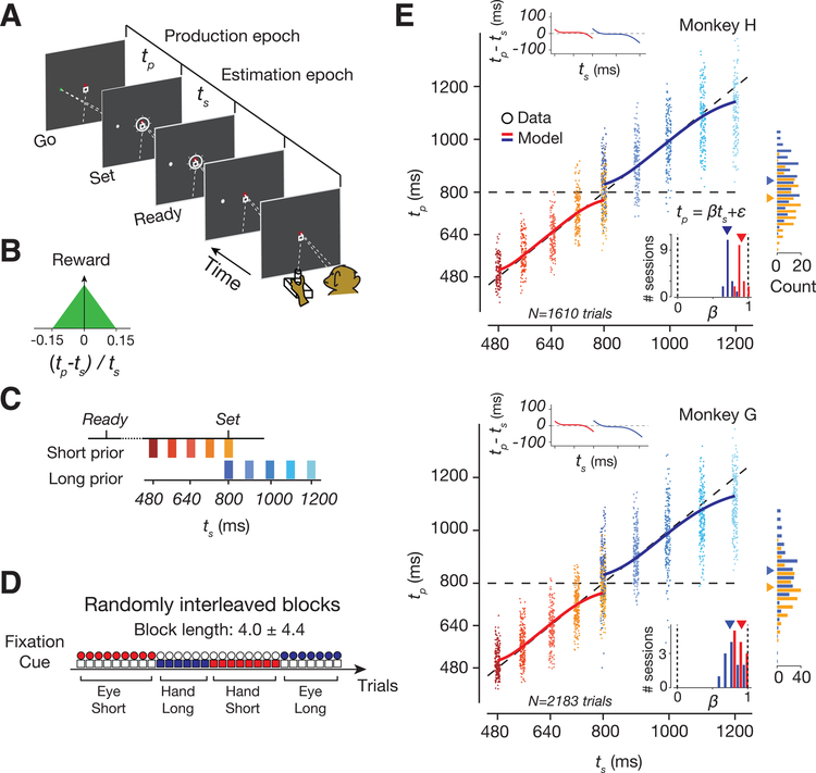
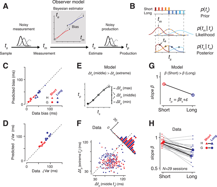
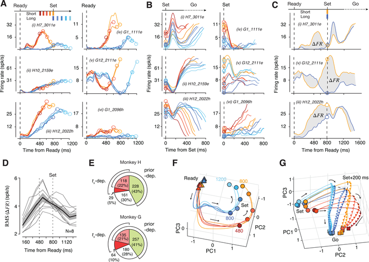
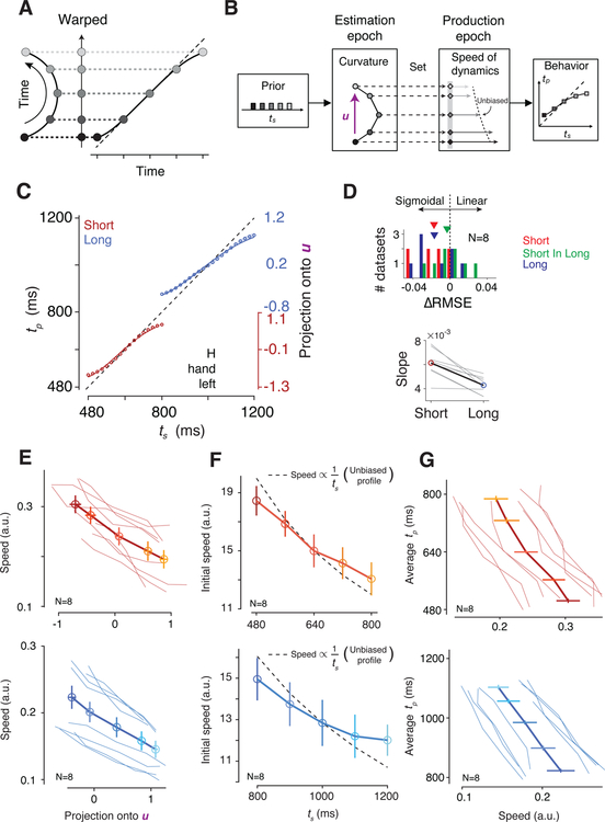
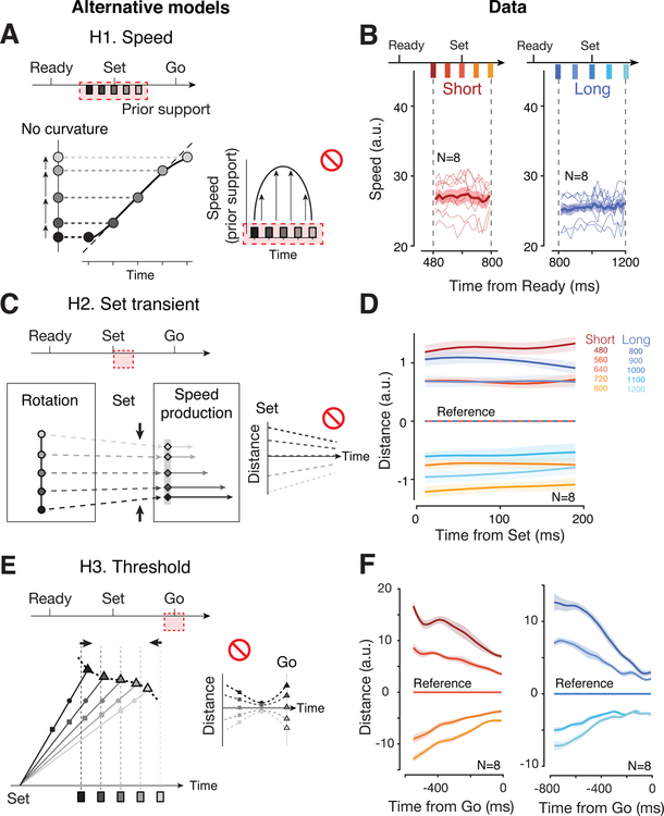
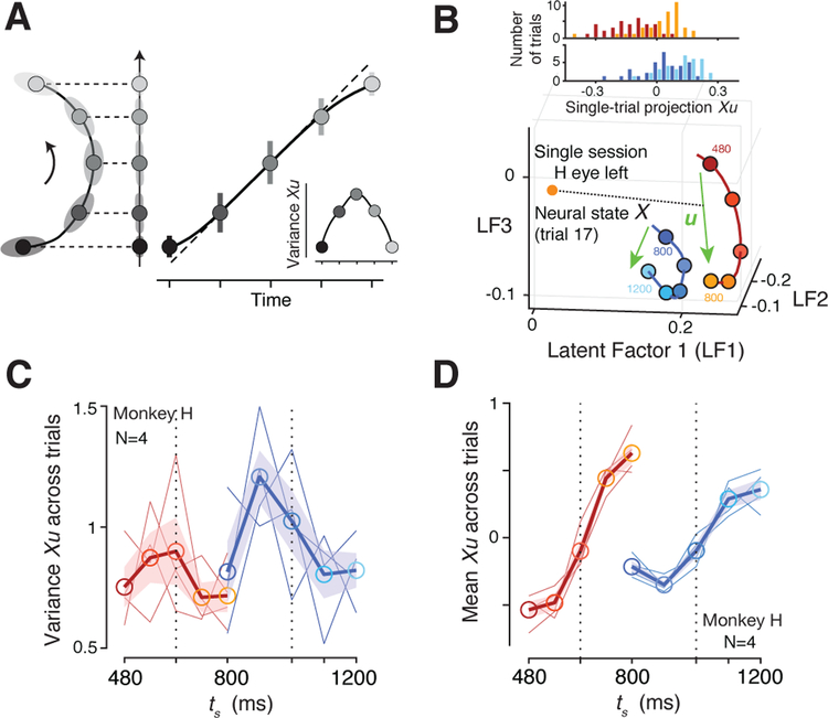
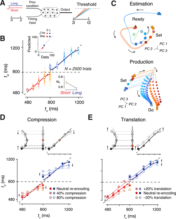
Statistical regularities in the environment create prior beliefs that we rely on to optimize our behavior when sensory information is uncertain. Bayesian theory formalizes how prior beliefs can be leveraged and has had a major impact on models of perception, sensorimotor function, and cognition. However, it is not known how recurrent interactions among neurons mediate Bayesian integration. By using a time-interval reproduction task in monkeys, we found that prior statistics warp neural representations in the frontal cortex, allowing the mapping of sensory inputs to motor outputs to incorporate prior statistics in accordance with Bayesian inference. Analysis of recurrent neural network models performing the task revealed that this warping was enabled by a low-dimensional curved manifold and allowed us to further probe the potential causal underpinnings of this computational strategy. These results uncover a simple and general principle whereby prior beliefs exert their influence on behavior by sculpting cortical latent dynamics.

Keywords: Bayesian inference; Bayesian integration; frontal cortex; neural manifold; neural trajectories; recurrent neural networks.


Conflict of interest statement

Declaration of Interests

The authors declare no competing interests.

Figures

Figure 1.
Figure 1.. Task and behavior.
(A) Schematic of a single trial of the Ready-Set-Go task. The animal has to estimate a sample interval, ts, between Ready and Set (estimation epoch), and produce a matching interval, tp, after Set with a delayed response (Go) via a saccade or a movement of the joystick (production epoch). (B) Reward as a function of relative error (tp-ts)/ts. (C) ‘Short’ and ‘Long’ prior distributions of ts. (D) Eight randomly interleaved trial types (see Methods): 2 prior conditions (Short and Long) × 2 effectors (Eye and Hand) × 2 target directions (Left and Right). (E) Behavior. Top: A representative session for monkey H showing tp pooled across effectors and target directions (small dots: individual trials; large open circles: average tp per ts; solid lines: Bayesian model; diagonal: unity line). The horizontal location of dots was jittered to facilitate visualization. Right: Histograms of tp for the overlapping ts (horizontal dashed line) for the two prior conditions (orange: Short; blue:Long; triangles: averages). Top-left inset: Average error (i.e., bias) for each ts (circles: data; solid lines: Bayesian model). Bottom-right inset: histogram of regression slopes relating tp to ts across sessions (red: Short; blue: Long; triangles: averages). Bottom: The same as top for Monkey G.
Figure 2.
Figure 2.. Bayesian model and behavior.
(A) Bayesian observer model. The measurement (tm) is the sample interval (ts) plus white noise with standard deviation proportional to ts. The Bayesian estimator is a sigmoidal function that maps tm to an optimal estimate (te) (red: Short; blue: Long). te is biased toward the mean of the prior (arrows). The production interval (tp) is te plus scalar noise during production epoch. (B) The prior (top), the likelihood function (middle), the resulting posterior (bottom), and the posterior mean (circles) that represent the estimate. (C) Comparison of tp bias relative to ts between model and behavior across animals and conditions. (D) Same as C for variability. Individual trials were pooled across sessions for each condition to compute the variance. (E) The sigmoidal Bayesian estimator predicts that the average tp difference across neighboring ts (∆tp) should be larger around the mean of the prior distribution (∆tp(middle)), compared to its extrema, ∆tp (extreme) (average of ∆tp(max) and ∆tp(min)). (F) ∆tp (extreme) as a function ∆tp (middle) for each session and condition (prior, response modality, direction) pooled across the two monkeys. Each data point represents a session (red: Short; blue: Long). Top-right: Histogram of the difference between ∆tp(middle) and ∆tp(extreme). The difference was similar between Short and Long (red and blue triangles) as predicted by the model. Triangles shows averages across datasets. See also Figure S1. (G) Model prediction for bias for the two prior conditions. (H) Slopes of regression lines relating tp to ts for individual sessions (small markers connected by gray lines), and the corresponding averages (big markers connected by a black line). Triangles represent monkey H, and circles, monkey G.
Figure 3.
Figure 3.. DMFC response profiles and neural trajectories.
(A) Firing rate of 6 example neurons (i-vi) during the estimation epoch for Short (shades of red) and Long (shades of blue) prior conditions aligned to the time of Ready (vertical dashed line), and Set (open circles). Top left: the support of the prior. Labels (e.g., H7_3011e) indicate the animal (H versus G) and the effector (e for Eye and h for Hand). (B) Same as A during the production epoch. Due to animals’ behavioral variability, production epochs for the same ts were of different durations. The plot shows the average activity of neurons from the time of Set (vertical dashed line) to the minimum tp for each ts. (C) Firing rate of 3 of the neurons in panel A throughout the trial for the overlap ts of 800 ms (Short: orange, Long: blue). The shaded area shows the difference in firing rates between the two prior conditions (∆FR). (D) Root-Mean-Squared (RMS) of ∆FR during the trial (bin size: 160 ms; thin gray line: data from 2 animals × 2 effectors × 2 directions; thick black line: mean across 8 datasets; shaded area: s.e.m.). (E) Pie chart of the percentage of neurons with activity dependent on the prior (“prior-dep.”) and/or ts (“ts-dep.”), determined by a generalized linear model (green: only prior-dependent, dark red: only ts-dependent, light red: both prior- and ts-dependent, white: the remaining neurons). (F) Neural trajectories during the estimation epoch for a representative dataset (Monkey H, Eye Left condition) in the subspace spanned by the first three principal components (PCs) with the same color scheme as panel A (triangles: Ready; circles: Set; arrows: temporal evolution of trajectories). (G) Same as F for the production epoch (circles: Set; squares: Go). Trajectories were truncated at the minimum tp for each ts (dashed line: neural states 200 ms after Set; small dots: neural states at 20-ms increments). The distance between consecutive dots reflects speed. See Figure S3 for other datasets.
Figure 4.
Figure 4.. Neural signatures of Bayesian integration.
(A) A geometric illustration of how linear projection of points along a 2D curve onto a 1D line could cause sigmoidal nonlinearity (gray dashed lines). (B) The cascade of computations during the Ready-Set-Go task for different sample intervals (ts). The prior distribution of ts (leftmost panel) establishes curved trajectory during the estimation epoch (second leftmost panel). Projection of neural states along the curved trajectory onto an encoding axis (purple vector, u) creates a warped 1D representation of time that exhibits prior-dependent biases. In the ensuing production epoch (after the presentation of Set), the initial conditions (second rightmost panel; gray diamonds) reflect the warped representation of time and lead to biased speed profiles (dotted line: unbiased speed profile with 1/ts, see panel F). The biased speed profiles, in turn, allow the system to exhibit Bayes-optimal behavior (rightmost panel). (C) Projection of neural states in the estimation epoch onto the encoding axis (u) as a function of ts for a representative condition (Monkey H, Hand Left condition) along the Bayesian model fit to behavior (line). Projections onto u (right ordinate axis) were linearly mapped onto the tp range (left ordinate axis) with two free parameters for scaling and offset (circles: projections every 20 ms; red: Short; blue: Long; shaded area: 95% bootstrap confidence intervals). (D) Top: The difference between Root-Mean-Squared-Error (∆RMSE) of the Bayesian and linear model fits with the same number of free parameters (red: Short; blue: Long; green: Short in Long, see main text). Triangles at top show mean ∆RMSE averaged across individual datasets (2 animals × 2 effectors × 2 directions) for each prior condition. Bottom: regression slope relating neural projections to ts for the Short and Long prior conditions (gray lines: individual datasets; black line with colored circles: mean). (E) Speed of neural trajectories from Set to Go as a function of the projection of the neural state at Set onto u. The speed was estimated by averaging distances between successive bins of the states in the state space (thin lines: individual datasets across animals and conditions; thick line: average). Error bars are s.e.m. (F) Speed profile across ts within each prior. The dashed line represents the unbiased speed profile; we used the middle speed as reference, and scaled it according to each interval assuming constant travelling distance. To ensure that speed biases were already present early in the production epoch, speeds were computed as the average speed between Set and Set+400ms (i.e., initial speed). Results are presented in the same format as in E. (G) Average produced interval (tp) as a function of speed at which neural states evolved during the production epoch. Results are presented in the same format as in E.
Figure 5.
Figure 5.. Alternative mechanisms.
(A) Speed model (H1). Top: Bayesian estimation during the support of the prior (shaded red) through modulation of speed. Bottom: If speed of neural trajectory is modulated according to an inverted U-shape (accelerating then decelerating; right), projections off of the trajectory would exhibit regression to the mean (gray dashed lines). (B) Instantaneous speed of neural trajectories during the estimation epoch for Short (red) and Long (blue) prior conditions computed in the full neural state space (thin lines: individual conditions for each animal; thick line: averages; shaded regions: s.e.m.) Speeds were relatively constant during the support of the prior and did not follow the pattern predicted by H1. (C) Transient model (H2). Top: Bayesian estimation through transient responses triggered by Set (shaded red). Bottom: The Set flash could pushes the system along slightly converging trajectories across ts causing regress to the mean. This predicts a reduction of distance between consecutive trajectories shortly after Set (right). (D) Distance between neural trajectories during the first 200 ms following Set. For each prior, we used the trajectory associated with the middle ts as reference (horizontal lines at y=0). For each time point along the reference trajectory, we computed the distance to the four other trajectories within each prior (shaded regions: s.e.m. across datasets). Trajectories were analyzed using PCA between Set and Set+200ms across the two prior conditions (>75% variance explained). Distance were relatively fixed and did not converge as predicted by H2. (E) Threshold model (H3). Top: Bayesian estimation through adjustment of threshold at the time of Go (shaded red). Bottom: If action-triggering states (curved dashed line) are biased such that faster trajectories (i.e., associated with shorter ts) have to travel longer distances to reach the threshold, threshold-crossing times (triangles) would exhibit regression to the mean even with unbiased speeds (left). This predicts a distinctive nonmonotonic organization of neural trajectories: distances between trajectories associated with different ts exhibit a large-small-large (squares-circles-triangles) pattern before the Go response (right). (F) Distance between neural trajectories aligned to the motor response. Similar to D, we used the middle trajectory as reference for the two prior conditions (left for Short, right for Long). Distances decreased monotonically and did not follow the distinctive pattern predicted by H3. Shaded area represents 95% confidence interval across conditions and animals. Distances were computed in the PC space obtained across ts and accounting for ~60% of the total variance; results remained unchanged when more PCs were included. See also Figure S5.
Figure 6.
Figure 6.. Trial-by-trial analyses.
(A) A geometric interpretation of how a curved neural trajectory could establish the bias-variance trade-off expected from the sigmoidal Bayesian estimator in our task. Curvature causes neural states near the two ends to be mapped onto a relatively narrow range (smaller error bars). This squashes variability of neural projections (Xu) and predicts an inverted-U profile for variance as a function of ts (inset). (B) Single-trial estimate of neural states (X). Bottom: Neural trajectories during the support of the Short (red) and Long (blue) prior conditions based on neural state estimates derived from a Gaussian process factor analysis (GPFA; see Methods). Top: Neural states for each ts projected onto the encoding axis (u). (C) Variance of projected neural states (Xu) across ts. We z-scored Xu of all trials before computing the variance for each ts (thin lines: individual conditions; thick line: averages across conditions; shaded area: s.e.m. across conditions). (D) Projected neural states averaged across single-trials as a function of ts for both priors. See also Figure S6.
Figure 7.
Figure 7.. Recurrent neural network model of Bayesian integration.
(A) Schematic of RNN experimental design. RNN received two inputs. One provides a tonic input encoding the prior condition (Short: red; Long: blue), and the other supplies two pulses representing Ready (R) and Set (S). The network was trained to generate a linearly ramping output whose slope was inversely related to the sample interval between R and S (ts). The Go response (G) was elicited when the output reached a threshold (dashed line). The production interval (tp) was measured as the time between S and G. (B) Network behavior shown using the same format as in Figure 1E. Inset top: Bias (circles) and variance (triangles) of network responses compared to that of a Bayesian model for the Short (red) and Long (blue) prior conditions using the same procedure as Figure 2C,D. Inset bottom: Regression coefficient analysis for the two priors (same color scheme) for different network runs. (C) Network unit trajectories shown using the same format as Figure 3F,G. (D) Top: Schematic showing perturbed states (white circle) that are compressed toward the state associated with the mean ts (arrows) relative to the original states (gray circles). Bottom: Network behavior with no compression (dark hue, neutral re-encoding), with 40% compression (intermediate hue, and with 80% compression (light hue) for the Short (red) and Long (blue) prior conditions. Solid lines represent corresponding fits to the Bayesian model. (E) Same as D for translational perturbation with either 20% positive translation along the moving trajectory or 20% negative translation against the moving trajectory. Solid lines represent the Bayesian model translated by an offset. See also Figure S7.

Similar articles

Cited by

References

    1. Acerbi L, Wolpert DM, and Vijayakumar S (2012). Internal representations of temporal statistics and feedback calibrate motor-sensory interval timing. PLoS Comput. Biol 8, e1002771. - PMC - PubMed
    1. Afshar A, Santhanam G, Yu BM, Ryu SI, Sahani M, and Shenoy KV (2011). Single-trial neural correlates of arm movement preparation. Neuron 71, 555–564. - PMC - PubMed
    1. Akrami A, Kopec CD, Diamond ME, and Brody CD (2018). Posterior parietal cortex represents sensory history and mediates its effects on behaviour. Nature 554, 368–372. - PubMed
    1. Angelaki DE, Gu Y, and DeAngelis GC (2009). Multisensory integration: psychophysics, neurophysiology, and computation. Curr. Opin. Neurobiol 1–7. - PMC - PubMed
    1. Athalye VR, Ganguly K, Costa RM, and Carmena JM (2017). Emergence of Coordinated Neural Dynamics Underlies Neuroprosthetic Learning and Skillful Control. Neuron 93, 955–970.e5. - PubMed

Publication types

LinkOut - more resources