Human foveal cone photoreceptor topography and its dependence on eye length

Abstract

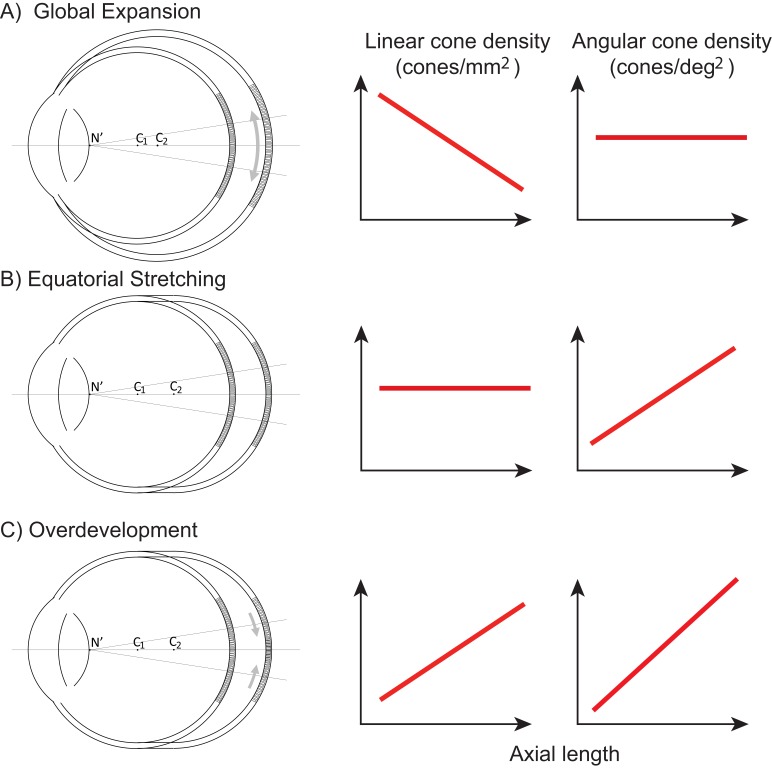
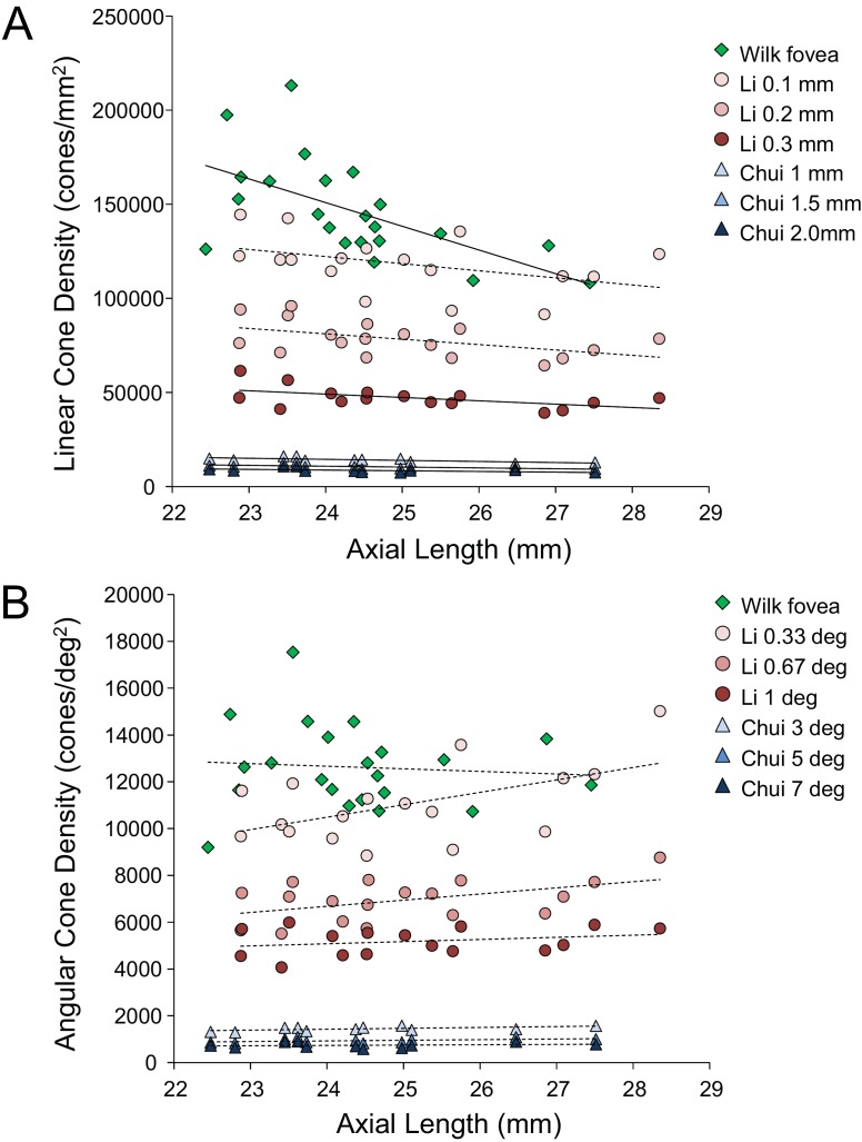
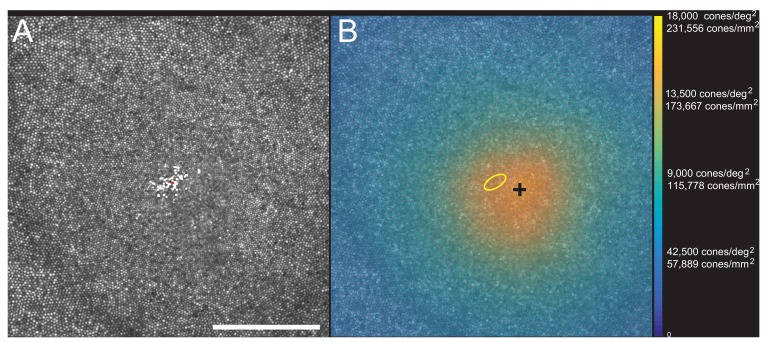
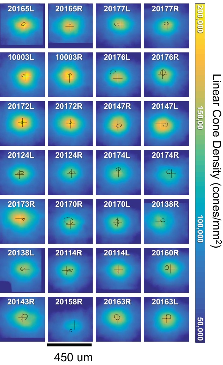
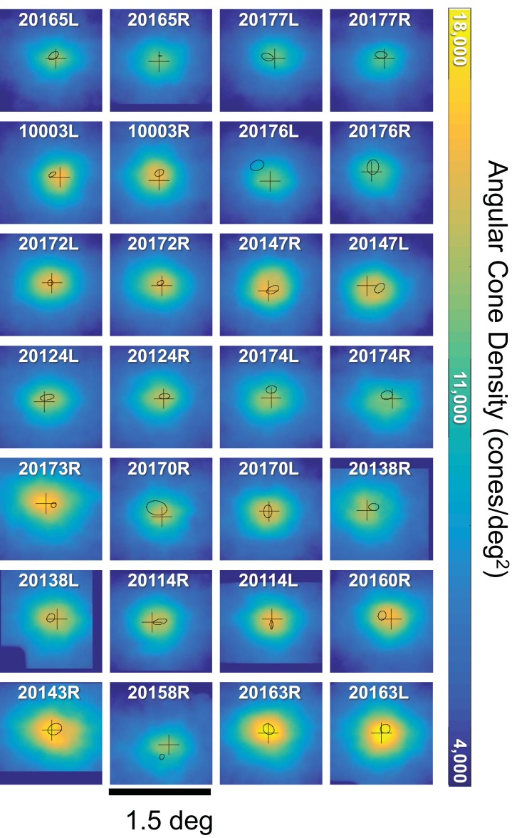
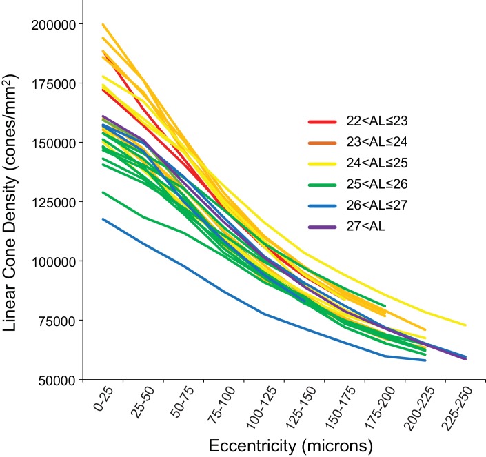
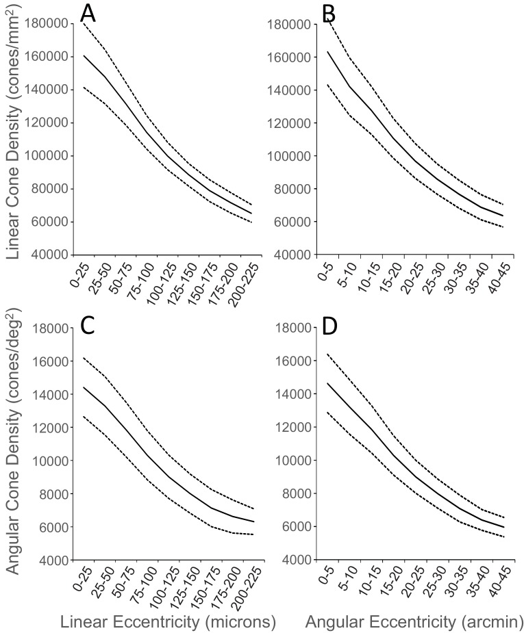
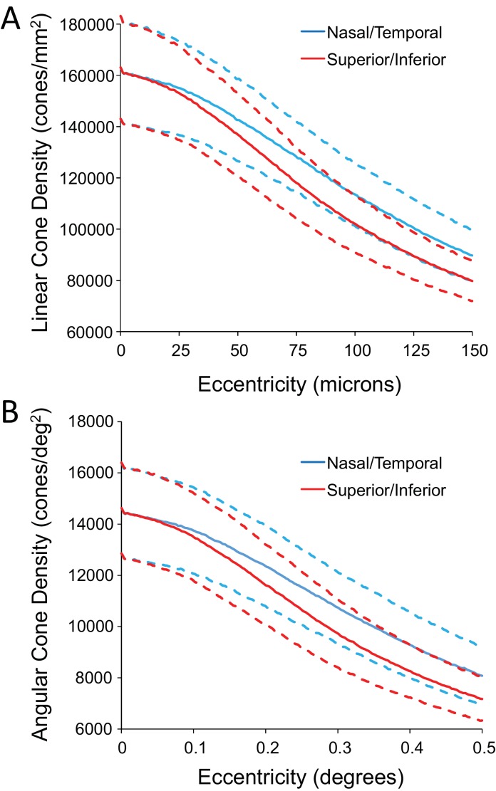
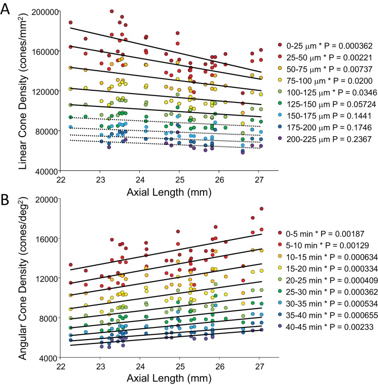
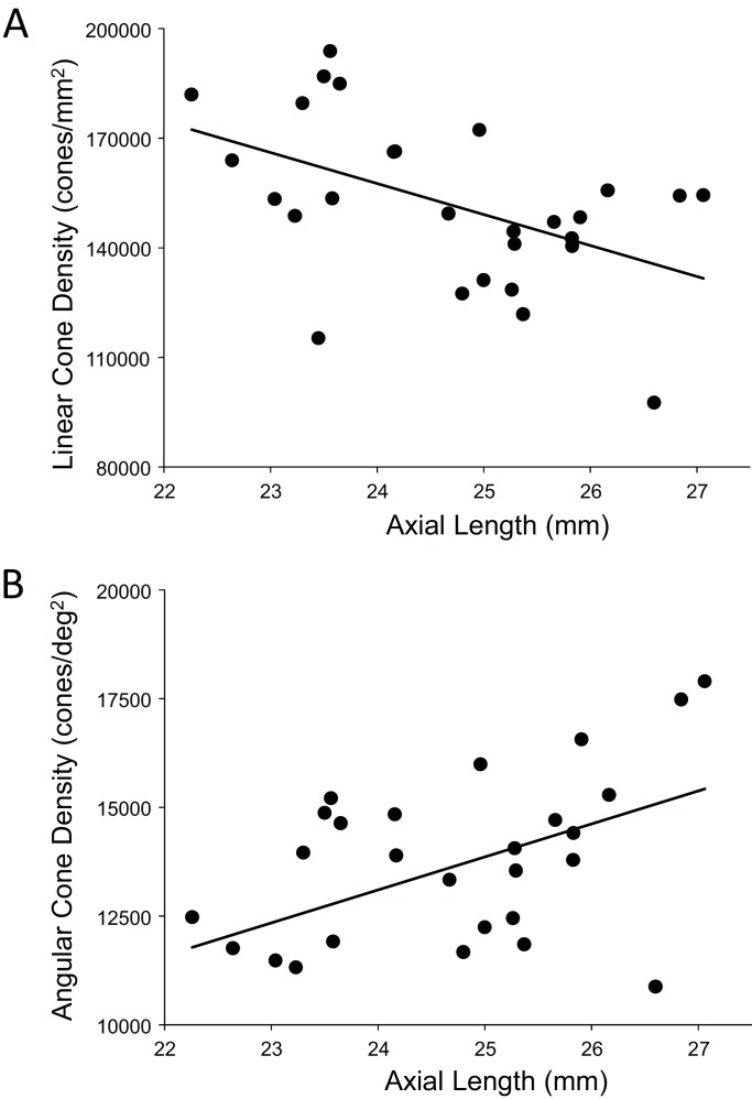
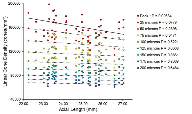
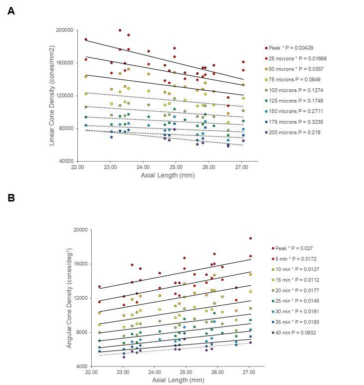
We provide the first measures of foveal cone density as a function of axial length in living eyes and discuss the physical and visual implications of our findings. We used a new generation Adaptive Optics Scanning Laser Ophthalmoscope to image cones at and near the fovea in 28 eyes of 16 subjects. Cone density and other metrics were computed in units of visual angle and linear retinal units. The foveal cone mosaic in longer eyes is expanded at the fovea, but not in proportion to eye length. Despite retinal stretching (decrease in cones/mm²), myopes generally have a higher angular sampling density (increase in cones/deg²) in and around the fovea compared to emmetropes, offering the potential for better visual acuity. Reports of deficits in best-corrected foveal vision in myopes compared to emmetropes cannot be explained by increased spacing between photoreceptors caused by retinal stretching during myopic progression.

Keywords: adaptive optics; cone photoreceptors; fovea; human; myopia; neuroscience.

Figure 1.. Three models of myopic eye growth.

(A) Global expansion shows an eyeball that is proportionally stretched. (B) The equatorial stretching model indicates a growth model where the fovea stays rigid and unaffected as the eye grows. (C) The over-development model shows that myopic eye growth is similar with developmental eye growth where photoreceptors continue to migrate towards the fovea as the eye grows.

Figure 2.. Summary of published data from Li et al. (2010), Chui et al. (2008) and Wilk et al. (2017).

In both plots, the linear fits with the solid lines indicate the data that have significant trends. (A) Linear cone density has a decreasing trend with axial length near the fovea. (B) Angular cone density (sampling resolution) of the eye generally increases with axial length although none of the data show a significant linear relationship.

Figure 3.. Image, PRL, cone locations and density plot for one subject.

(A) AOSLO image of the fovea of subject 10003L. Only the central 1.5 degrees are shown here (810 × 810 pixels), which contains 16,184 cones. The white dots are a scatter plot showing the PRL, or position of the fixated stimulus over the course of a 10 s video. The red dot is the centroid of the scatter plot. (B) Same image with a color overlay indicating the density. Linear and angular cone densities are indicated on the right colorbar. Peak cone densities in this eye are 204,020 cones/mm² and 15,851 cones/deg². The yellow ellipse is the best fitting ellipse containing ~68% of the points in the scatterplot and indicates the PRL. The black cross indicates the position of peak cone density. Scale bar is 0.5 degrees, which in this eye corresponds to 139.4 microns.

Figure 3—figure supplement 1.. Linear cone density (cones/mm²) plots over the central 450 microns for all 28 eyes.

The black cross indicates the point of maximum cone density. The black ellipse is the best fitting ellipse about the fixation scatterplot indicating the PRL. Dark blue regions indicate where no cone density estimates were made.

Figure 3—figure supplement 2.. Angular cone density (cones/deg²) plots over the central 1.5 degrees for all 28 eyes.

The black cross indicates the point of maximum cone density. The black ellipse is the best fitting ellipse about the fixation scatterplot indicating the PRL. Dark blue regions indicate where no cone density estimates were made.

Figure 4.. Cone density as a function of eccentricity for all eyes.

The axial length ranges of the subjects are color coded, with warmer colors for shorter eyes and cooler colors for longer eyes. In this plot, it is apparent that shorter eyes generally have higher peak cone densities.

Figure 4—figure supplement 1.. Plots of average cone density of all 28 eyes as a function of eccentricity in units of.

(A) cones/mm² vs. eccentricity in microns, (B) cones/mm² vs. eccentricity in arcminutes (C) cones/deg² vs. eccentricity in microns and (D) cones/deg² vs. eccentricity in arcminutes. The solid lines are the average and the upper and lower dashed lines represent ±1 standard deviation from the average.

Figure 4—figure supplement 2.. Plots of density as a function of eccentricity in the vertical and horizontal directions.

(A) linear cone density (B) angular cone density. The dashed lines represent ±1 standard deviation from the mean.

Figure 5.. Plots of cone density as a function of axial length at and near the fovea.

(A) Linear cone densities as a function of axial length. Longer eyes have lower linear cone density than shorter eyes. The trend remains significant out to 100 microns eccentricity. At the peak, the details for the trendline are: slope = −3,185 with 95% confidence intervals from −4,578 to −13,793. (B) Angular cone densities as a function of axial length. The peak angular cone density increases significantly with increasing axial length and this trend remains significant out to 40 arcminutes eccentricity. At the peak, the details for the trendline are: slope = 749 with 95% confidence intervals from 304 to 1193. Relationships with p-values<0.05 are labeled with asterisks and trendlines are shown as solid lines. Relationships with p-values≥0.05 have dashed trendlines.

Figure 6.. The relationship between cone density and axial length shows the same pattern at the PRL as for the peak cone density.

The numbers for the trendline in (A) are slope: 759; 95% CI: 198 to 1,320; p=0.00999. The numbers for the trendline in (B) are: slope = −8,490; 95% CI −14,600 to −2,420; p=0.00795). Axial length accounts for 24%% and 23% of the variance in linear and angular cone density, respectively.

Figure 7.. Plots of the magnitude of fixational eye movements as a function of axial length.

(A) The plot of BCEA in linear units (square microns) vs. axial length shows a trend that approaches significance (p=0.0596). (B) There is no significant relationship between BCEA in angular units (square arcminutes) and axial length (p=0.364).

Author response image 1.. Plots of linear cone density at different retinal locations using retinal magnification factors computed using a formula from Bennett et.al., 1994.

Even though the retinal image size for myopes is underestimated for myopes and overestimated for hyperopia, there is still a significant drop in density with increasing axial length at the location of peak density.

Author response image 2.. Changes in linear and angular cone density with axial length over a range of distances from the location of peak density.

The results for one eye are essentially the same as that reported in the paper.

Author response image 3.. The right plot shows that the peak foveal cone density increases as the cone sampling window is decreased.

Note that the increase with reducing sampling window is linear until about 10 arcminutes. The left plot shows that the variability in the location of the peak foveal density remains consistent (within about 1.5 arcminutes of the mean) with cone sampling windows of 10 arcminutes or greater.

References

1. Agaoglu M, Sit MT, Wan D, Chung ST. GitHub; 2018. https://github.com/lowvisionresearch/ReVAS
1. Atchison DA, Jones CE, Schmid KL, Pritchard N, Pope JM, Strugnell WE, Riley RA. Eye shape in Emmetropia and myopia. Investigative Opthalmology & Visual Science. 2004;45:3380–3386. doi: 10.1167/iovs.04-0292. - DOI - PubMed
1. Atchison DA, Schmid KL, Pritchard N. Neural and optical limits to visual performance in myopia. Vision Research. 2006;46:3707–3722. doi: 10.1016/j.visres.2006.05.005. - DOI - PubMed
1. Bennett AG, Rudnicka AR, Edgar DF. Improvements on Littmann's method of determining the size of retinal features by fundus photography. Graefe's Archive for Clinical and Experimental Ophthalmology. 1994;232:361–367. doi: 10.1007/BF00175988. - DOI - PubMed
1. Bruce KS, Harmening WM, Langston BR, Tuten WS, Roorda A, Sincich LC. Normal perceptual sensitivity arising from weakly reflective cone photoreceptors. Investigative Opthalmology & Visual Science. 2015;56:4431–4438. doi: 10.1167/iovs.15-16547. - DOI - PMC - PubMed
Publication types