Accelerating structure-function mapping using the ViVa webtool to mine natural variation

Abstract

Thousands of sequenced genomes are now publicly available capturing a significant amount of natural variation within plant species; yet, much of these data remain inaccessible to researchers without significant bioinformatics experience. Here, we present a webtool called ViVa (Visualizing Variation) which aims to empower any researcher to take advantage of the amazing genetic resource collected in the Arabidopsis thaliana 1001 Genomes Project (http://1001genomes.org). ViVa facilitates data mining on the gene, gene family, or gene network level. To test the utility and accessibility of ViVa, we assembled a team with a range of expertise within biology and bioinformatics to analyze the natural variation within the well-studied nuclear auxin signaling pathway. Our analysis has provided further confirmation of existing knowledge and has also helped generate new hypotheses regarding this well-studied pathway. These results highlight how natural variation could be used to generate and test hypotheses about less-studied gene families and networks, especially when paired with biochemical and genetic characterization. ViVa is also readily extensible to databases of interspecific genetic variation in plants as well as other organisms, such as the 3,000 Rice Genomes Project ( http://snp-seek.irri.org/) and human genetic variation ( https://www.ncbi.nlm.nih.gov/clinvar/).

Keywords: Arabidopsis thaliana; accessibility; genome diversity; genotype‐phenotype; natural variation; structure‐function.

Figure 1

Rank order of the strength of functional effects variant effect classes were ordered by subjective prediction of average strength of effect on gene function. Strength was then assigned to each effect on an integer scale

Figure 2

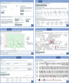
Key elements of the webtool (a) The first section contains two collapsible panels, gene select and annotation files, which are used to input information about the genes to be investigated. (b) The SNP Stats tab provides gene‐structure level counts and statistics on SNPs. (c) The Diversity Plot tab plots the nucleotide diversity of SNP sites along the length of the coding region of a selected gene. (d) The SNP Mapping tab plots accessions on a world map colored according to the selected set of SNPs. (e) The SNP Browser tab allows variants and accessions to be filtered by any combination of text and numeric fields. (f) The Alignments tab aligns DNA and amino acid sequences of homologous genes and colors sequence elements based on SNPs and annotations

Figure 3

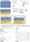
ViVa workflow (a) Workflow diagram of ViVa. Blue indicates user actions, yellow indicates processing steps performed by the application. (b) Detailed look at mapping tab parameters: User selects which genes to look at (1) then clicks the Submit button (2). The “Allele selection” panel is then filled in with all non‐reference variants meeting the criteria. The user can adjust the range of nucleotide diversity and the type of SNP with a slider and radio buttons (3) to make the list of variants a manageable size. The list of variants is updated as changes are made to these controls. The user then selects variants to display on the map (4). Clicking the Update Map button (5) populates the map below with points located at the collection coordinates of each accession and colored by the selected alleles. (c) Detailed look at the browser tab options: The user first selects which genes to analyze and clicks submit (1). The “hide 0|0 genotype?” checkbox (2) removes rows from the table containing the reference allele. Four configurable filters of two types are provided. The first filter type is text matching (3); the user selects a column to filter from a drop‐down menu then enters one or more text strings to match in that column. The second type of filter is numeric range matching (4); the user again selects a column, then specifies a range to match by typing or selecting minimum and maximum values. After configuring the filters, the user clicks the Apply Filters button (5) to update the table. The table is updated such that only rows that meet all filter conditions are displayed

Figure 4

IAA6 Diversity Plot. Nucleotide diversity of variant positions throughout the IAA6 coding sequence are plotted and colored according to the effect of the variant alleles at each position. The region of positive selection identified by Winkler et al. is highlighted

Figure 5

Map of AFB1 Oligomerization domain variant accessions. (a) Map showing the two accessions with variants in the AFB1 oligomerization domain (b) The user selectable parameters of the mapping tab used to generate the map are provided as an example of using the SNP Mapping tab in the ViVa webtool. See Figure 3 for details on filling in the parameters

Figure 6

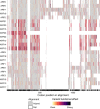
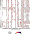
Critical functional domains of the conserved Aux/IAA genes show low nonsynonymous variation compared to regions of unknown functional importance. Protein sequences were aligned with DECIPHER (Wright, 2015) and variants were mapped to this alignment and colored according to the predicted functional effect of the allele of strongest effect at that position, with light colors having weaker effects on function and darker colors stronger effects. Red indicates missense variants. Color scale is further explained in Section 2. Alignment consensus is shown in grayscale underneath the plot as measured by evolutionary trace (Płuciennik et al., 2018; Wilkins, Erdin, Lua, & Lichtarge, 2012), with high consensus positions in black and low consensus in white. Key functional domains are outlined in black and labeled above the plot. The EAR domain spans codon alignment positions 70–74, corresponding to IAA1 amino acids LRLGL, 14–18. The degron domain spans alignment positions 194–201, corresponding to IAA1 amino acids QIVGWPPV, 55–62. The charged residues of the PB1 domain correspond to alignment positions 246, 256, 316, 318, 320, and 326 corresponding to IAA1 amino acids K77, R88, D133, D135, D137, and D143

Figure 7

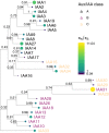
IAA protein sequence phylogenetic tree mapped with π_N/π_S reveals patterns of sister pair diversity/conservation. Protein sequences were aligned with DECIPHER (Wright, 2015) and low‐information content regions were masked with Aliscore (Kück et al., 2010) prior to inferring a phylogeny with MrBayes (Ronquist & Huelsenbeck, 2003). Tips of the tree are mapped with circles of color and diameter proportional to π_N/π_S. π_N/π_S statistic provides a prediction of functional diversity. Nodes are labeled with the posterior probability of monophyly, a measure of confidence in the branch assignment, with one representing high confidence and zero, low confidence. There are two distinct clades of Aux/IAAs represented by the majority of the A and B classes. C class Aux/IAAs are missing one or more of the canonical Aux/IAA domains. These classes are represented by the text color of the gene name

Figure 8

Auxin‐signaling F‐box protein sequence tree mapped with π_N/π_S. Protein sequences were aligned with DECIPHER (Wright, 2015) and low‐information content regions were masked with Aliscore (Kück et al., 2010) prior to inferring a phylogeny with MrBayes (Ronquist & Huelsenbeck, 2003). Tips of the tree are mapped with circles of diameter proportional to π_N/π_S. Nodes are labeled with the posterior probability of monophyly

Figure 9

Alignment of the auxin‐signaling F‐box family protein sequences were aligned with DECIPHER (Wright, 2015) and variants were mapped to this alignment and colored according to the predicted functional effect of the allele of strongest effect at that position, with light colors having weaker effects on function and darker colors stronger effects. Red indicates missense variants. Color scale is explained in Section 2. In grayscale underneath the plot, alignment consensus is shown as measured by evolutionary trace (Płuciennik et al., 2018; Wilkins et al., 2012), with high‐consensus positions in black and low consensus in white

Figure 10

TPL protein sequence tree mapped with π_N/π_S. Protein sequences were aligned with DECIPHER (Wright, 2015) and low‐information content regions were masked with Aliscore (Kück et al., 2010) prior to inferring a phylogeny with MrBayes (Ronquist & Huelsenbeck, 2003). Tips of the tree are mapped with circles of diameter proportional to π_N/π_S and also are colored according to π_N/π_S. Nodes are labeled with the poster probability of monophyly

Figure 11

Alignment of the TPL/TPR family. Protein sequences were aligned with DECIPHER (Wright, 2015) and variants were mapped to this alignment and colored according to the predicted functional effect of the allele of strongest effect at that position, with light colors having weaker effects on function and darker colors stronger effects. Red indicates missense variants. Color scale is explained in Section 2. In grayscale underneath the plot, alignment consensus is shown as measured by evolutionary trace (Płuciennik et al., 2018; Wilkins et al., 2012), with high‐consensus positions in black and low consensus in white

Figure 12

Auxin response factor protein sequence tree mapped with π_N/π_S. Protein sequences were aligned with DECIPHER (Wright, 2015) and low‐information content regions were masked with Aliscore (Kück et al., 2010) prior to inferring a phylogeny with MrBayes (Ronquist & Huelsenbeck, 2003). Tips of the tree are mapped with circles of diameter proportional to π_N/π_S and also are colored according to π_N/π_S. Nodes are labeled with the poster probability of monophyly

Figure 13

Alignment of the full auxin response factor family. Protein sequences were aligned with DECIPHER (Wright, 2015) and variants were mapped to this alignment and colored according to the predicted functional effect of the allele of strongest effect at that position, with light colors having weaker effects on function and darker colors stronger effects. Red indicates missense variants. Color scale is explained in Section 2. In grayscale underneath the plot, alignment consensus is shown as measured by Evolutionary trace (Płuciennik et al., 2018; Wilkins et al., 2012), with high‐consensus positions in black and low consensus in white

Figure 14

Alignment of the complete Aux/IAA family. Protein sequences were aligned with DECIPHER (Wright, 2015) and variants were mapped to this alignment and colored according to the predicted functional effect of the allele of strongest effect at that position, with light colors having weaker effects on function and darker colors stronger effects. Red indicates missense variants. Color scale is further explained in Section 2. Alignment consensus is shown in grayscale underneath the plot as measured by evolutionary trace (Płuciennik et al., 2018; Wilkins et al., 2012), with high‐consensus positions in black and low consensus in white

References

1. Alexandre, C. M. , Urton, J. R. , Jean‐Baptiste, K. , Huddleston, J. , Dorrity, M. W. , Cuperus, J. T. , … Queitsch, C. (2018). Complex relationships between chromatin accessibility, sequence divergence, and gene expression in Arabidopsis thaliana . Molecular Biology and Evolution, 35(4), 837–854. 10.1093/molbev/msx326 - DOI - PMC - PubMed
1. Allaire, J. J. , Ushey, K. , & Tang, Y. (2018). Reticulate: Interface to ‘Python’. Retrieved from https://CRAN.R-project.org/package=reticulate
1. Allaire, J. J. , Xie, Y. , McPherson, J. , Luraschi, J. , Ushey, K. , Atkins, A. , … Iannone, R. (2018). Rmarkdown: Dynamic documents for R. Retrieved from https://CRAN.R-project.org/package=rmarkdown
1. Aphalo, P. J. (2018a). Gginnards: Explore the innards of ‘Ggplot2’ objects. Retrieved from https://CRAN.R-project.org/package=gginnards
1. Aphalo, P. J. (2018b). Ggpmisc: Miscellaneous extensions to ‘Ggplot2’. Retrieved from https://CRAN.R-project.org/package=ggpmisc
LinkOut - more resources