. 2019 Aug 2;15(8):e1007205.
doi: 10.1371/journal.pcbi.1007205. eCollection 2019 Aug.

Bayesian hypothesis testing and experimental design for two-photon imaging data

Affiliations

Bayesian hypothesis testing and experimental design for two-photon imaging data

Luke E Rogerson et al. PLoS Comput Biol. .

Erratum in

Abstract

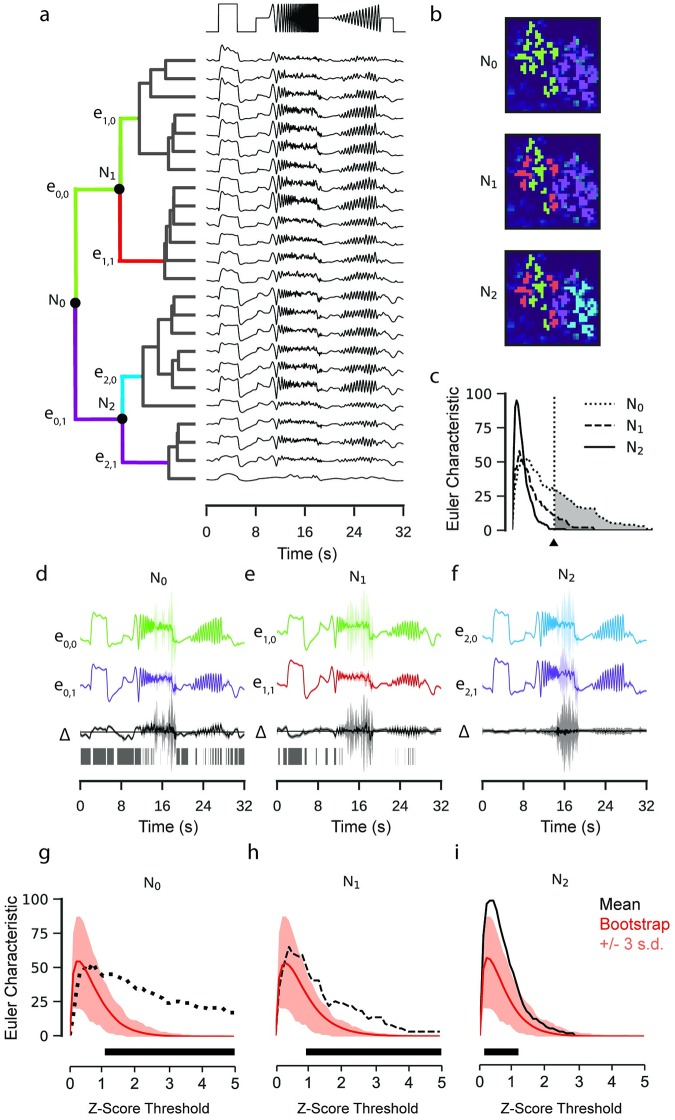
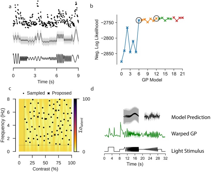
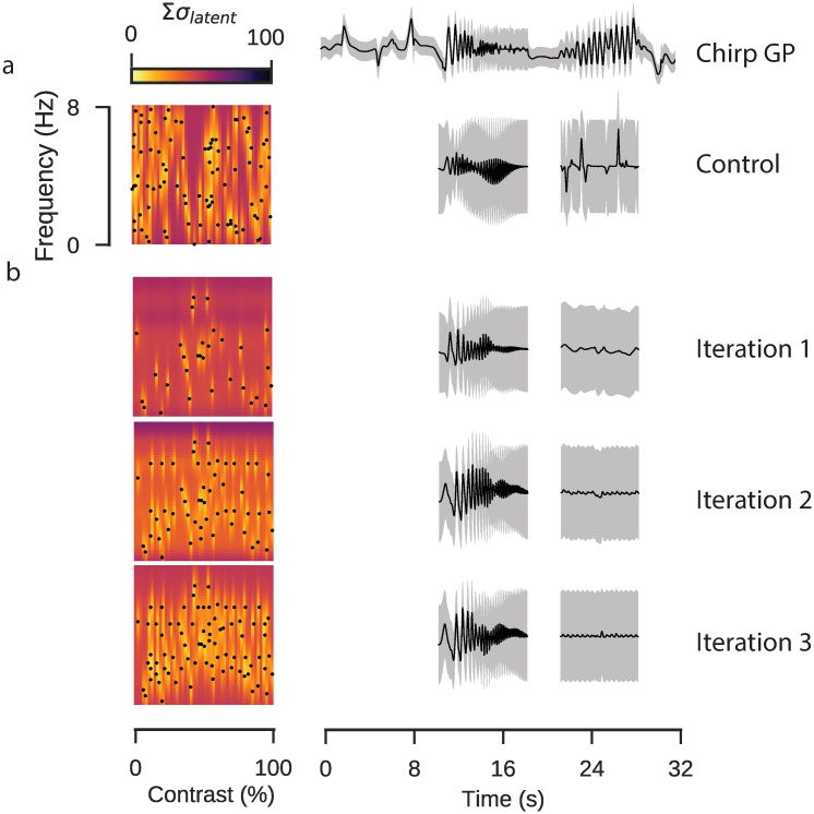
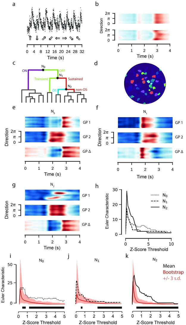
Variability, stochastic or otherwise, is a central feature of neural activity. Yet the means by which estimates of variation and uncertainty are derived from noisy observations of neural activity is often heuristic, with more weight given to numerical convenience than statistical rigour. For two-photon imaging data, composed of fundamentally probabilistic streams of photon detections, the problem is particularly acute. Here, we present a statistical pipeline for the inference and analysis of neural activity using Gaussian Process regression, applied to two-photon recordings of light-driven activity in ex vivo mouse retina. We demonstrate the flexibility and extensibility of these models, considering cases with non-stationary statistics, driven by complex parametric stimuli, in signal discrimination, hierarchical clustering and other inference tasks. Sparse approximation methods allow these models to be fitted rapidly, permitting them to actively guide the design of light stimulation in the midst of ongoing two-photon experiments.


Conflict of interest statement

The authors have declared that no competing interests exist.

Figures

Fig 1
Fig 1. Two-photon imaging of retinal neurons.
Data: Retinal bipolar cell filled with OGB-1 via sharp electrode injection and recorded using linear and spiral scan configurations. a: Vertical profile. Image coloured according to fluorescence intensity (yellow: high, blue: low). b: Horizontal (x-y), high-resolution scan of axon terminal system (512 x 512 pixels), corresponding to the domain between the two white ticks in (a). c: Spiral scan of axon terminal system (16 spirals; 31.25 Hz), as above. d: Linear scan of axon terminal system (32 lines; 15.625 Hz), as above. e: Spiral scan trajectory with ROI mask superimposed. Black lines indicate scan trajectory. Colours correspond to discrete ROIs. f: As (e), but with a linear scan configuration. The same ROIs were used. g: Time points at which the scan trajectory intersects with the ROI mask in (e). 64 ms span corresponds to two spiral scan frames. h: As (g), but for a linear scan configuration. ROIs correspond to those in (f). 64 ms span corresponds to one linear scan frame.
Fig 2
Fig 2. Inference of signals from two-photon data.
Data: ROI from a retinal bipolar cell filled with OGB-1 via sharp electrode injection (left), and a different ROI from a scan field with bipolar cell terminals in a retina expressing iGluSnFR (right); both recorded using spiral scan configurations. Model: RBF kernel, 300 inducing inputs, 25 iterations per fit, best of 6 fits per model. a: “Full-field chirp” light stimulus, consisting of a light step, a frequency-modulated sine wave and a contrast-modulated sine wave. b: Observed activity of a single ROI. Each point corresponds to the mean activity of the ROI in a single scan line. The time at which the point was recorded is defined relative to the start of each stimulus trial, such that each trial leads to at least one data point for every time the laser scans across a given ROI. Information regarding the trial from which the point was derived is not explicitly incorporated into the model. c: Estimate of underlying signal from frame averaging, cubic spline interpolation and averaging over trials. This corresponds to the typical approach used in previous papers [7]. d: Fitted sparse Gaussian process. Black line indicates the mean signal. Intervals indicate uncertainty of the signal with and without the observation noise (light and dark grey, respectively), to 3 standard deviations. e: Fitted sparse warped Gaussian process. Input warping uses the warping function shown in the following figure. Model has been projected back onto the original time dimension. f: Five posterior samples drawn from the fitted sparse warped Gaussian process models.
Fig 3
Fig 3. Application of a warping function to model input features.
Data: ROI from a retinal bipolar cell filled with OGB-1 via sharp electrode injection. Model: RBF kernel, 300 inducing inputs, 20 iterations per fit, best of 3 fits per model. a: “Full-field chirp” stimulus (top). Autocorrelation functions corresponding to Gaussian curves fit to the empirical autocorrelation function over a 500 ms window (middle). Length scale parameter of the Gaussian distribution fitted to the autocorrelation functions. b: Cumulative sum of the inverse lengthscale over time. If the signal were stationary, the lengthscale would be constant, corresponding to the dashed line. This cumulative sum maps time onto a warped time dimension. c: Full field chirp stimulus with observations of the activity of one ROI labelled with OGB-1. d: The same stimulus and observations after a warping operation has been applied. e: GP fitted to the original data. f: GP fitted to the warped data. The function has been projected back onto un-warped time. Note the increased uncertainty in regions where the stimulus is changing rapidly and the variations in the smoothness of the inferred signal over time.
Fig 4
Fig 4. Gaussian process equality testing.
Data: ROI from a retinal bipolar cell filled with OGB-1 by sharp electrode injection (left), and a different ROI from a scan field with bipolar cell terminals in a retina expressing iGluSnFR (right); both recorded using spiral scan configurations. Model: GP w. Time Warp: RBF kernel, 300 inducing inputs, 20 iterations per fit, best of 5 fits per model. Classical: pipeline incorporating frame averaging and interpolation. a: “Chirp” light stimulus. b: Fits of the GP with time warping and classical pipeline to chirp-driven responses, for calcium and glutamate data. Models fitted to observations of the responses to local (100 μm; top) and full field (middle) chirp stimulus. Circles indicate relative spatial extent of the light stimulus. Difference between the models for the two stimulus conditions shown at the bottom. Intervals for the response data show 3 standard deviations above and below the mean function. This variability corresponds to the standard deviation with and without additive noise for the GPs, and the inter-trial standard deviation for the classical pipeline. Only the standard deviation without additive noise is shown for the difference of the GPs. Domains where zero-vector not included within this interval are highlighted with grey ticks, corresponding to regions where the difference between the two signals is greater than expected by chance. c: Frequency of discrete domains where zero-vector is not included in the credible intervals (also known as the Euler Characteristic; EC) as a function of the number of standard deviations above and below the respective mean functions. A high EC indicates a large degree of statistical separation between the two signals, and typically declines as the threshold increases. Bootstrap estimates of the null distribution of the EC are superimposed, with the mean of the null distributed shown in red. Intervals correspond to three standard deviations above and below the mean of the null distribution. The black box indicates the thresholds where the EC from the difference test exceeds the highest estimate from the null distribution by three standard deviations.
Fig 5
Fig 5. Hierarchical clustering of retinal bipolar cell terminals.
Data: ROIs from a retinal bipolar cell filled with OGB-1 by sharp electrode injection recorded using a linear scan configuration. Model: RBF kernel (time), 300 inducing inputs, 20 iterations per fit, best of 3 fits per model. One model fitted for each ROI. a: Mean functions of GP models fitted to calcium activity in a single recording field. Dendrogram computed using the Ward’s hierarchical clustering algorithm (left). Nodes where the equality test were performed are labelled N. Colours on the dendrogram correspond to putative clusters. b: ROI masks overlaid on mean field activity, coloured with respect to the putative cluster. Each overlay is coloured according to the clustering at the corresponding nodes in (a). c: Euler Characteristic for each node with respect to the z-score threshold. d, e, f: GP Equality tests performed at each of the labelled nodes. GPs correspond to the models fitted to each putative cluster (top, middle) and the difference between the two models (bottom). Intervals correspond to 3 standard deviations above and below mean function. Domains where zero-vector not included within interval highlighted with grey ticks. g, h, i: Bootstrap estimates of the null distribution of the Euler Characteristic (EC). Mean of null distributed shown in red. Intervals correspond to three standard deviations above and below the mean of the null distribution. Estimated EC from (c) superimposed. The black box indicates the thresholds where the EC from the difference test exceeds the highest estimate from the null distribution.
Fig 6
Fig 6. Extended GP model incorporating stimulus parameters.
Data: ROI from a scan field with bipolar cell terminals in a retina expressing iGluSnFR, recorded using a spiral scan configuration. Model: Product of RBF kernel (time) with composite RBF kernels (frequency and contrast), 500 inducing inputs, 50 iterations per fit, best of 5 fits per model. a: Observed activity of one ROI filled with OGB-1 (top); GP model selected by model selection procedure, conditioned on the observations of the ROI. Sine stimulus activity. Data corresponds to the first 9s of the stimulus. b: Negative log likelihood for each model tested during model selection. Each point corresponds to a single model, where the kernel consists of the effects adopted in the previous pass, with an additional effect being evaluated, which will be included if it has the highest negative log likelihood. Each “Pass” corresponds to an exhaustive evaluation of all possible effects to add to the current kernel. The best performing model in each pass is highlighted with a black circle. c: Locations in frequency-contrast parameter space selected for the stimulation. Colour map corresponds to the sum of the variance of the latent function for the fitted GP model evaluated under each parameter combination. Crosses correspond to peaks in the uncertainty where the stimulus should next be evaluated. Dashed line indicates the limits of the space from which the parameters were sampled. d: GP fitted to observed chirp responses for the same ROI (middle). Prediction of the activity by the model on the sine stimulus data (top).
Fig 7
Fig 7. Active parameter selection with Gaussian processes.
Data: ROI from a scan field with bipolar cell terminals in a retina expressing iGluSnFR, recorded using a spiral scan configuration. Model: Product of RBF kernel (time) with composite RBF kernels (frequency and contrast), 500 inducing inputs, 50 iterations per fit, best of 4 fits per model. a: Control stimulus consisting of 90 parameter sets of frequency and contrast. Uncertainty in each region computed as the sum of the latent uncertainty for a GP estimated under all parameter configurations. The chirp response for this ROI is shown above. The completed GP model for the sine response is estimated over the full dataset, the model inference for the sinusoidal chirp components is shown. b: Active parameter selection using GP with corresponding inferences for chirp stimulus.
Fig 8
Fig 8. GP model of retinal ganglion cell responses to a moving bar stimulus.
Data: ROIs from a field of RGC somata labelled with OGB-1 using electroporation, recorded using a spiral scan configuration. Model: Product of RBF kernel (time) with composite RBF kernel (direction), 300 inducing inputs, 25 iterations per fit, best of 3 fits per model. a: Observed activity of one ROI representing an RGC soma labelled with OGB-1 (top). GP model superimposed. Intervals correspond to the variance of the latent function, 3 standard deviations above and below the mean. Below are the moving bar directions for each trial. b: GP model fitted to data in (a) without (top) and with (bottom) interaction kernel. Both models include additive effects for direction and time. Coloured according to response amplitude (red: high, blue: low). c: Hierarchical clustering of fitted models. Colours on dendrogram correspond to colours on ROI mask. Posterior means for each ROI in each cluster are shown in S2 Fig. d: ROI mask with cluster colours for k = 4 corresponding to clustering in (c). A baseline s.d. was computed from the 500 ms of activity preceding the light step. ROIs where the amplitude of the step response was less than 2 s.d. greater or lower than the mean signal were excluded. e, f, g: GP Equality Tests for each node. Top and middle correspond to the two putative clusters, bottom is the mean difference between them. h: Euler Characteristic as a function of the number of standard deviations above and below the respective mean functions, for each node. i, j, k: Euler Characteristics (EC) from difference tests at the first three nodes, with bootstrap estimates of the null distribution of the EC superimposed. The mean of the null distributed shown in red. Intervals correspond to three standard deviations above and below the mean of the null distribution. The black bar indicates the thresholds where the EC from the difference test exceeds the highest estimate from the null distribution by three standard deviations.

Similar articles

Cited by

References

    1. Denk W, Strickler JH, Webb WW. Two-photon laser scanning fluorescence microscopy. Science. 1990;248(4951):73–76. - PubMed
    1. Faisal AA, Selen LPJ, Wolpert DM. Noise in the nervous system. Nature reviews neuroscience. 2008;9(4):292 10.1038/nrn2258 - DOI - PMC - PubMed
    1. Wilt BA, Fitzgerald JE, Schnitzer MJ. Photon shot noise limits on optical detection of neuronal spikes and estimation of spike timing. Biophysical journal. 2013;104(1):51–62. 10.1016/j.bpj.2012.07.058 - DOI - PMC - PubMed
    1. Rasmussen CE, Williams CKI. Gaussian processes for machine learning. Cambridge, MA: MIT Press; 2006.
    1. Titsias M. Variational Learning of Inducing Variables in Sparse Gaussian Processes. Proceedings of the International Conference on Artificial Intelligence and Statistics (AISTATS). 2009;5:567–74.

Publication types

MeSH terms