Machine Learning Allows Calibration Models to Predict Trace Element Concentration in Soils with Generalized LIBS Spectra

Abstract

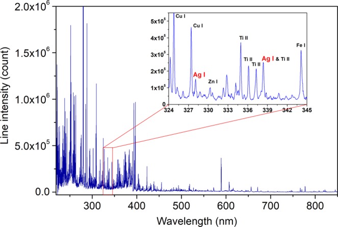
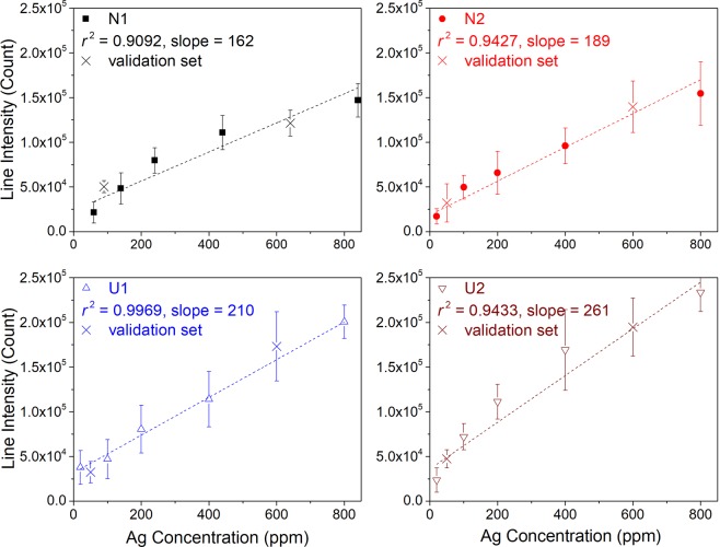
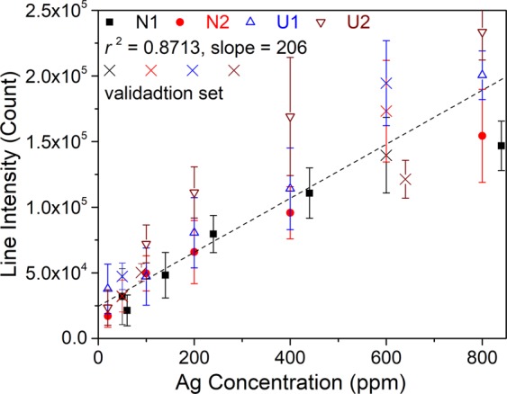
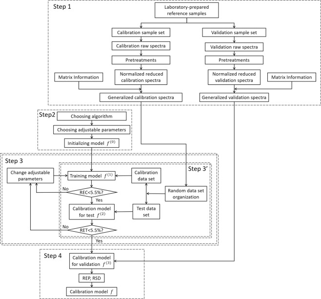
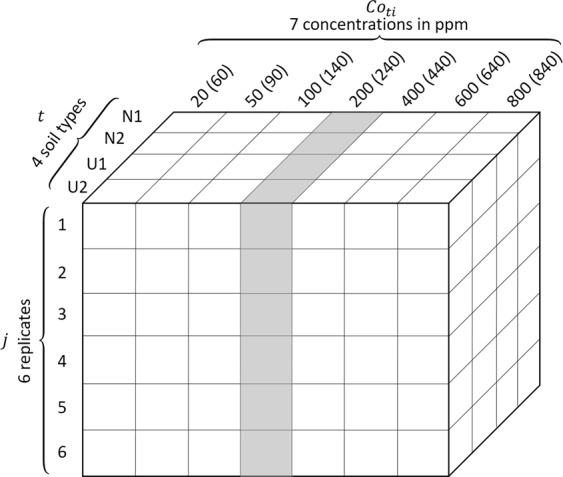
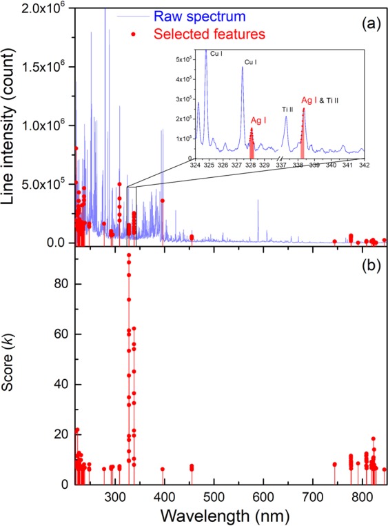
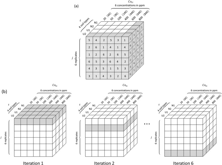
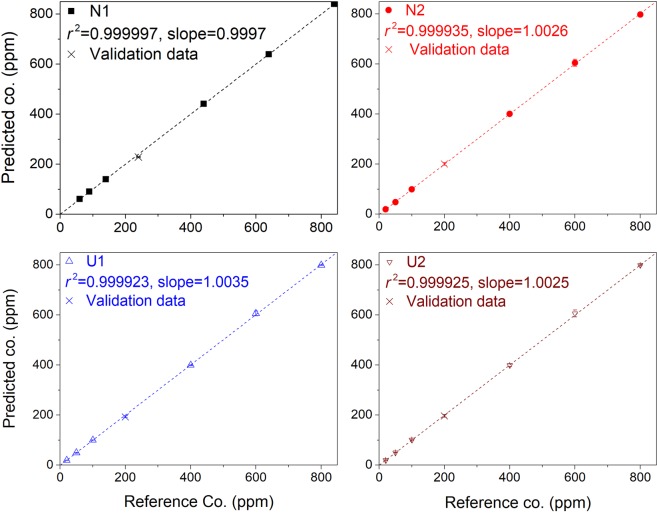
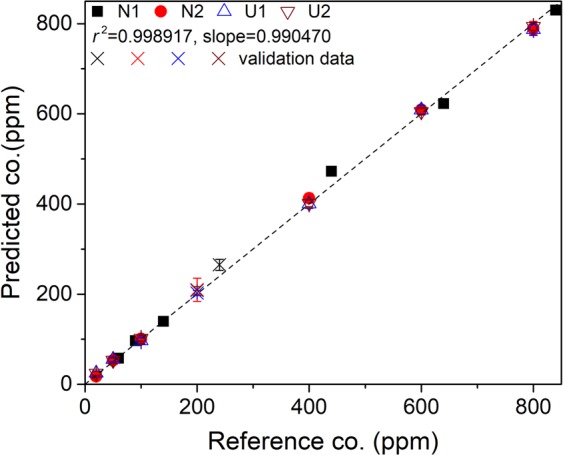
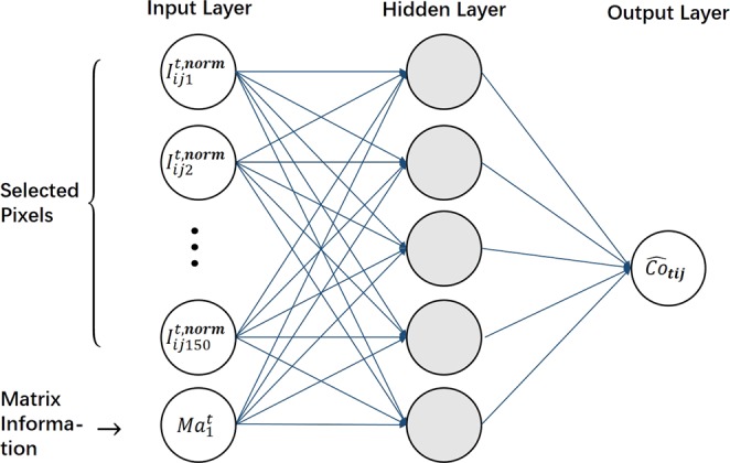
Determination of trace elements in soils with laser-induced breakdown spectroscopy is significantly affected by the matrix effect, due to large variations in chemical composition and physical property of different soils. Spectroscopic data treatment with univariate models often leads to poor analytical performances. We have developed in this work a multivariate model using machine learning algorithms based on a back-propagation neural network (BPNN). Beyond the classical chemometry approach, machine learning, with tremendous progresses the last years especially for image processing, is offering an ensemble of powerful and constantly renewed algorithms and tools efficient for the different steps in the construction of a spectroscopic data treatment model, including feature selection and neural network training. Considering the matrix effect as the focus of this work, we have developed the concept of generalized spectrum, where the information about the soil matrix is explicitly included in the input vector of the model as an additional dimension. After a brief presentation of the experimental procedure and the results of regression with a univariate model, the development of the multivariate model will be described in detail together with its analytical performances, showing average relative errors of calibration (REC) and of prediction (REP) within the range of 5-6%.

Figure 1

Typical replicate-averaged spectrum of soil sample. In the inset, the detailed spectrum around the Ag I 328.1 nm line is shown. Sample used to obtain the spectrum: t = N1, initially containing the following elements: Cu (3420 ppm), Zn (4180 ppm), Ti (3110 ppm), Fe (43200 ppm), and Ag (40 ppm), 400 ppm of Ag was additionally spiked into the sample (Co_ti = 440 ppm).

Figure 2

Intensities of Ag I 328.1 nm line of the calibration samples as function of Ag concentrations and soil-specific univariate calibration curve (dashed lines in the figures) of Ag with this line respectively for the 4 analyzed soils. Line intensities from the validation set are represented by crosses, they do not participate in the construction of the calibration models. The error bars are calculated for each line intensity with the standard deviation among the 6 replicate measurements ($\pm {\sigma }_{I_i^t}$).

Figure 3

Similar presentation of the experimental data as in Fig. 2, but with line intensities from all the 4 soils merged in a same figure and a soil-independent univariate calibration curve (dashed line).

Figure 4

Flowchart for the buildup of the multivariate calibration model. The steps contained in double dashed line rectangles are repeated within a conditional loop.

Figure 5

Structure of the experimental data with 4 soil types (t), 7 analyte concentrations (Co_ti) for each soil type and 6 replicate LIBS measurements (j) for a sample pellet of given soil type and analyte concentration. The samples with 200 (240) ppm analyte concentration are chosen as the validation sample set, the rest as the calibration sample set.

Figure 6

(a) Spectrum of the selected features (in red) with in the inset, those corresponding to the 2 Ag I lines, the raw spectrum (in light blue) is also shown for comparison; (b) Spectrum of the SelectKBest scores.

Figure 7

(a) A randomly and independently arranged data configuration among (6!)²⁴ possible and statistically equivalent ones; (b) For a given randomly and independently arranged data configuration, illustration of a 6-fold cross-validated training iteration, with the cubes in grey representing the test data set.

Figure 8

Model-predicted Ag concentrations as function of the prepared ones and soil-specific calibration curves for Ag concentration based on the multivariate calibration models. Validation data are represented in the figures with crosses.

Figure 9

Model-predicted Ag concentrations as a function of the prepared ones and soil-independent calibration curve for Ag concentration based on the multivariate calibration model. Validation data are represented in the figure with crosses.

Figure 10

Structure of the used neural networks.

References

-
- Mallarino, A. P. Testing of soils. in Encyclopedia of soils in the environment, 143–143 (Elsevier, 2005).
- McGrath, S. P. Pollution/Industrial. in Encyclopedia of soils in the environment, 282–287 (Elsevier, 2005).
- Kirkby, E. A. Essential elements. in Encyclopedia of soils in the environment, 478–485 (Elsevier, 2005).
- Singh V, Agrawal HM. Qualitative soil mineral analysis by EDXRF, XRD and AAS probes. Radiat. Phys. Chem. 2012;81:1796–1803. doi: 10.1016/j.radphyschem.2012.07.002. - DOI
Grants and funding
- 11805126/National Natural Science Foundation of China (National Science Foundation of China)
- 11601327/National Natural Science Foundation of China (National Science Foundation of China)
- 11574209/National Natural Science Foundation of China (National Science Foundation of China)
- 15142201000/Science and Technology Commission of Shanghai Municipality (Shanghai Municipal Science and Technology Commission)
LinkOut - more resources
Full Text Sources
Other Literature Sources