Rigid Motion Correction for Brain PET/MR Imaging using Optical Tracking

Abstract

A significant challenge during high-resolution PET brain imaging on PET/MR scanners is patient head motion. This challenge is particularly significant for clinical patient populations who struggle to remain motionless in the scanner for long periods of time. Head motion also affects the MR scan data. An optical motion tracking technique, which has already been demonstrated to perform MR motion correction during acquisition, is used with a list-mode PET reconstruction algorithm to correct the motion for each recorded event and produce a corrected reconstruction. The technique is demonstrated on real Alzheimer's disease patient data for the GE SIGNA PET/MR scanner.

Fig. 1.

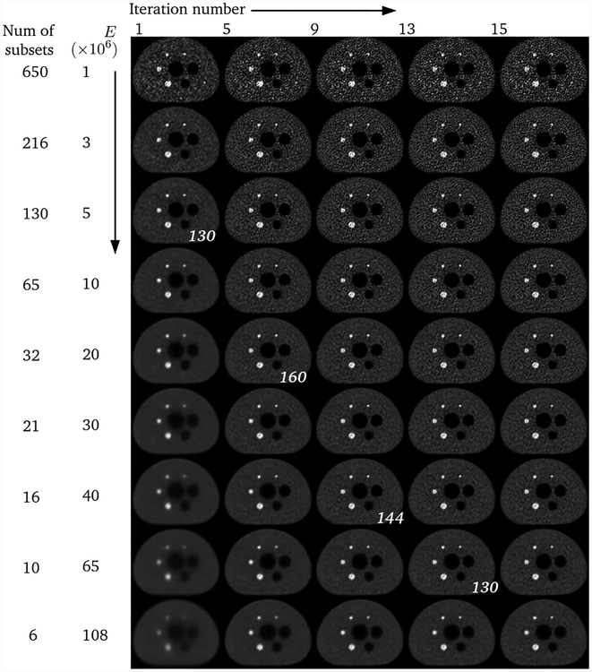
Each row shows a different reconstruction of the NEMA phantom data using increasing E (and therefore decreasing number of subsets), with increasing number of iterations for each reconstruction from left to right. The italicised numbers indicate reconstructions with similar number of updates, which should therefore be comparable in image quality.

Fig. 2.

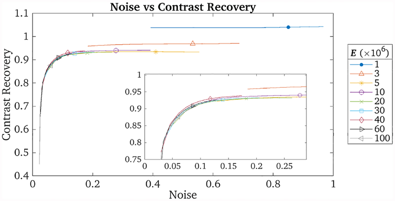
Plot of image noise versus contrast recovery for the 22 mm hot sphere for reconstructions with varying E. The symbols indicate the values at iteration 8. The inset shows that the plots for E ≥ 5 × 10⁶ all lie approximately on top of each other.

Fig. 3.

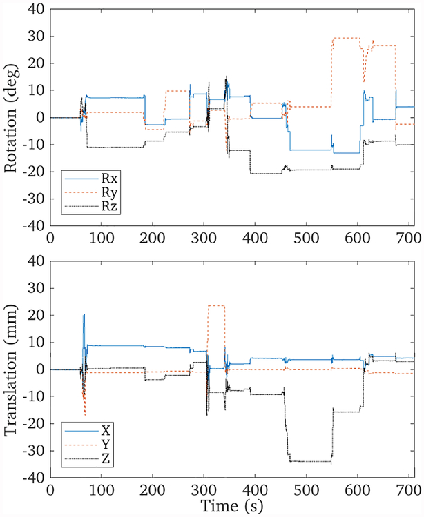
Tracked motion data of the three point sources over the 700 second scan. A large range of motion was exhibited

Fig. 4.

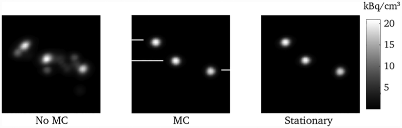
Maximum intensity projections of the reconstructions of the point source data. The left and middle reconstructions are of the same data set but without and with motion correction, respectively. The right reconstruction is of the stationary data set, whose position and orientation were used as a reference frame for the motion corrected reconstruction in the middle. The white lines indicate the locations of the profiles shown in figure 5.

Fig. 5.

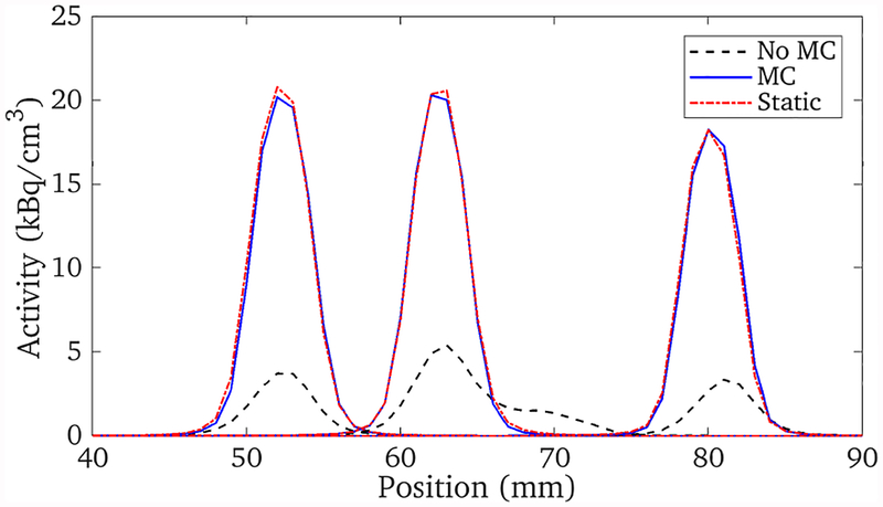
The profiles through the reconstructions shown in figure 4. The motion corrected and stationary data reconstructions agree with each other very closely.

Fig. 6.

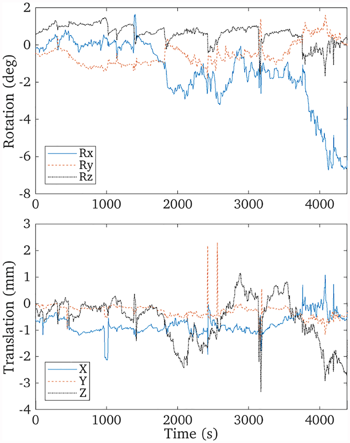
Tracked motion data of the patient brain scan over the 70 minute scan. Substantial motion can be observed in the last 10 minutes of the scan, corresponding to a nodding motion of the head.

Fig. 7.

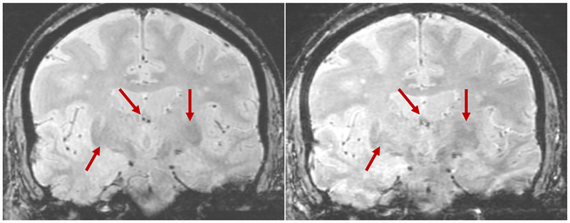
Comparing GRE images with (left, TR = 2500 ms) and without (right, TR = 2700 ms) motion correction (both: TE = 20 ms, FOV = 24 × 18 cm, slice thickness = 2 mm, inter-slice spacing = 0 mm, matrix = 384 × 256). The arrows indicate motion artefacts which are absent with motion correction.

Fig. 8.

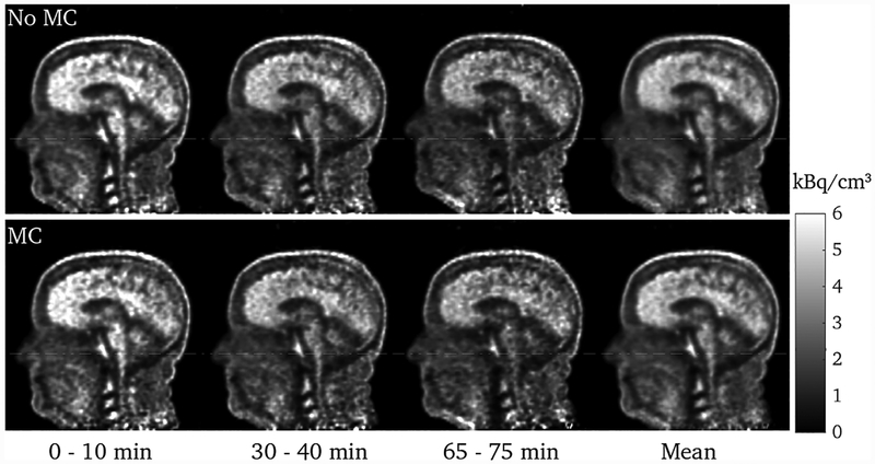
Sagittal slices through the head for frames at the beginning, middle, and end of the scan, and the mean of these three, without (top) and with (bottom) motion correction. The white dashed line is a visual guide. The motion is most evident by the lifting of the nose. The effect of the head motion has clearly been much reduced with motion correction.

Fig. 9.

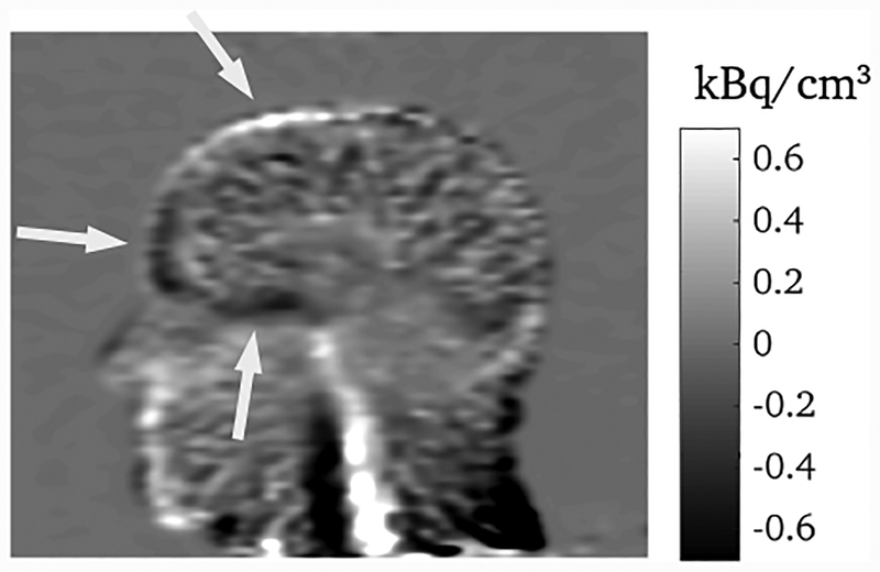
Difference image for the last 10 minute frame between the MC reconstruction and the non-MC reconstruction after it has been registered to the MC reconstruction. The differences in quantification indicated by the arrows are due to the mismatch between the emission data and the attenuation map in the non-MC reconstruction.

Fig. 10.

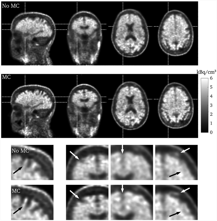
Sagittal, coronal, and two transverse slices through the brain for the entire scan duration, without (first row) and with (second row) motion correction. The bottom two rows show zoomed in sections of the images. The dashed lines indicate from where the slices are taken, and the red arrows highlight regions where the effect of the motion correction can be seen.

References

-
- Rahmim A, Bloomfield P, Houle S, Lenox M, Michel C, Buckley KR, Ruth TJ, and Sossi V, “Motion compensation in histogram-mode and list-mode EM reconstructions: beyond the event-driven approach,” IEEE Transactions on Nuclear Science, vol. 51, no. 5, pp. 2588–2596, 2004.
- Carson RE, Barker WC, Liow J-S, and Johnson CA, “Design of a motion-compensation OSEM list-mode algorithm for resolution-recovery reconstruction for the HRRT,” in IEEE Medical Imaging Conference Proceeding, vol. 5, 2003, pp. 3281–3285.
- Gillman A, Smith J, Thomas P, Rose S, and Dowson N, “PET motion correction in context of integrated PET/MR: Current techniques, limitations, and future projections,” Medical Physics, vol. 44, no. 12, pp. e430–e445, 2017. - PubMed
- Rahmim A, Rousset O, and Zaidi H, “Strategies for motion tracking and correction in PET,” PET clinics, vol. 2, no. 2, pp. 251–266, 2007. - PubMed
Grants and funding
LinkOut - more resources
Full Text Sources
Other Literature Sources