Displacement of a landslide retaining wall and application of an enhanced failure forecasting approach

Abstract

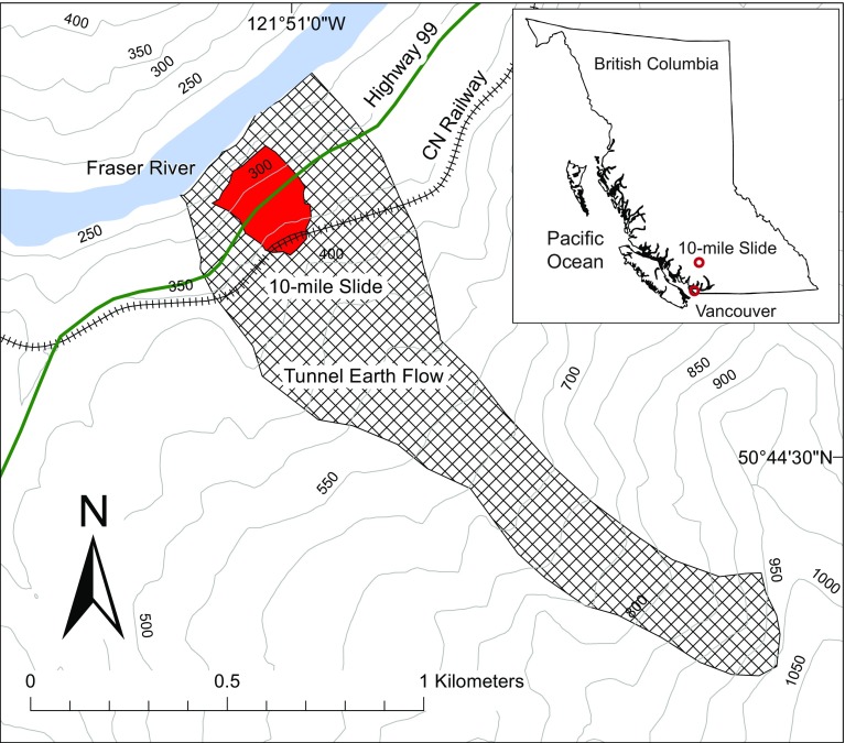
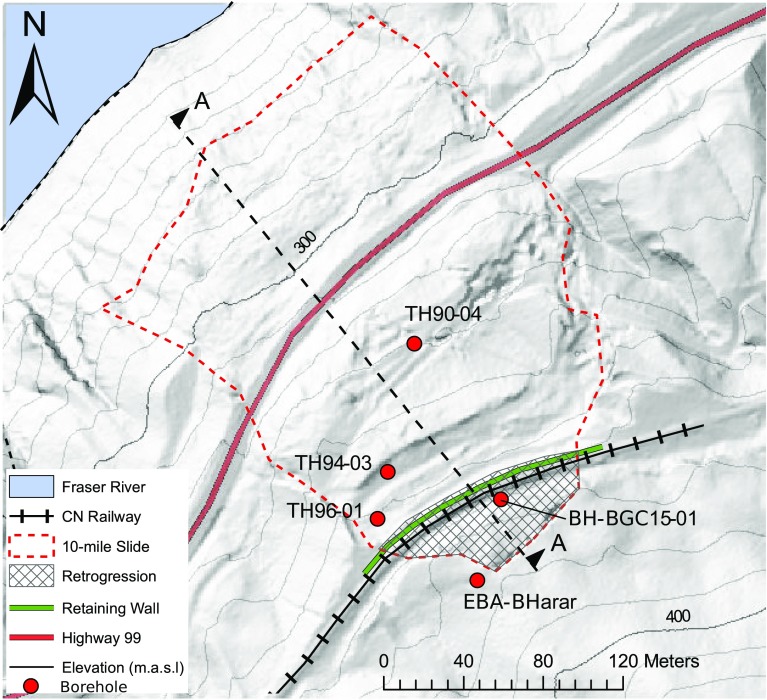
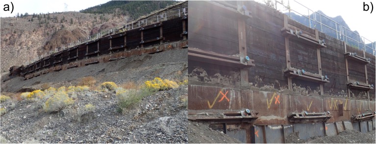
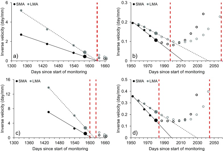
The 10-mile Slide is contained within an ancient earthflow located in British Columbia, Canada. The landslide has been moving slowly for over 40 years, requiring regular maintenance work along where a highway and a railway track cross the sliding mass. Since 2013, the landslide has shown signs of retrogression. Monitoring prisms were installed on a retaining wall immediately downslope from the railway alignment to monitor the evolution of the retrogression. As of September 2016, cumulative displacements in the horizontal direction approached 4.5 m in the central section of the railway retaining wall. After an initial phase of acceleration, horizontal velocities showed a steadier trend between 3 and 9 mm/day, which was then followed by a second acceleration phase. This paper presents an analysis of the characteristics of the surface displacement vectors measured at the monitoring prisms. Critical insight on the behavior and kinematics of the 10-mile Slide retrogression was gained. An advanced analysis of the trends of inverse velocity plots was also performed to assess the potential for a slope collapse at the 10-mile Slide and to obtain further knowledge on the nature of the sliding surface.

Keywords: Failure prediction; Inverse velocity; Landslide monitoring; Landslide retrogression; Retaining wall; Slope deformation analysis.

Fig. 1

Inverse velocity trends after onset of acceleration showing a a linear trend leading to slope failure and b an asymptotic trend leading to a steady state of constant deformation

Fig. 2

Conceptual model of failure window analysis: SMA represents displacement data filtered by means of a short-term moving average and LMA by means of a long-term moving average. The width of the failure window is calculated on the basis of the Δ between the LMA and SMA failure time predictions

Fig. 3

Location of the 10-mile Slide within the province of British Columbia and plan view of the landslide relative to the older, larger Tunnel earthflow. Highway 99 and CN’s railway are also shown (after Macciotta et al. ; Bovis 1985)

Fig. 4

Front view of the 10-mile Slide. Photo taken in July 2016

Fig. 5

Plan view of a shaded relief of the 10-mile Slide. Shaded relief corresponds to 2015 LiDAR imaging (after Macciotta et al. 2017a)

Fig. 6

Counter-slope scarps located between the railway track and Highway 99 (a), the uppermost tension crack observed above the railway track, as of April 2016 (b), and an 8- to 10-m-high scarp downslope from the railway track (c)

Fig. 7

Core material recovered from the landslide area at a depth between 14 and 16 m from the surface (a), detail of a sharp change between wet clayey till cohesive core and silty sand material with till inclusions (b), and core with heavily sheared till (c). After Macciotta et al. (2017b)

Fig. 8

Interpreted simplification of the cross-section of the 10-mile Slide (after Macciotta et al. 2017a)

Fig. 9

View of the retaining wall from the northernmost area of the landslide (a) and close view of the anchoring system (b)

Fig. 10

Sketch with the location of the retaining wall piles being monitored for displacement

Fig. 11

Time series of cumulative horizontal and vertical displacement of piles 0 and 6 (a), and of piles 13 and 14 (b) from February 2011 to September 2016. The two red dashed lines mark the onset of the first and second acceleration phase, respectively

Fig. 12

Velocities of piles 0 (a), 6 (b), 13 (c), and 14 (d) from February 2011 to September 2016

Fig. 13

Increments of horizontal displacement of selected central piles from January 2015 to March 2016 (left) and from April to September 2016 (right)

Fig. 14

Increments of horizontal displacement of selected lateral piles from January 2015 to March 2016 (left) and from April to September 2016 (right)

Fig. 15

Horizontal vs. vertical movements between January 2015 and September 2016 of piles 0 and 6 (a), and of piles 13 and 14 (b). In a, the black dashed lines represent movement over ideal surfaces of 20° and 30°, whereas the red dashed line over an ideal 23° surface

Fig. 16

Evolution of the azimuth angle of movement with time of the piles of the railway retaining wall. An azimuth of 0° indicates a perfectly northward direction of movement

Fig. 17

Evolution of the dip angle of movement with time of the piles of the railway retaining wall. A dip angle of 0° indicates a perfectly horizontal movement away from the slope

Fig. 18

a Horizontal velocity and b variation of azimuth angle with time of pile 15, showing a transition from Type 2 to Type 1 deformation behavior

Fig. 19

a Plot of inverse horizontal velocity of pile 0. b Plot of inverse vertical velocity of pile 0. c Plot of inverse horizontal velocity of pile 6. d Plot of inverse vertical velocity of pile 6. All plots are based on unfiltered data and highlight the two main landslide acceleration phases that occurred during the monitoring period.

Fig. 20

Failure window approach applied to inverse velocity data of pile 0. a First acceleration phase, horizontal direction. b Second acceleration phase, horizontal direction. c First acceleration phase, vertical direction. d Second acceleration phase, vertical direction. The red dashed lines define the limits of the failure window, the larger points mark days no. 1582 and 1980 (i.e., T _c), and the hollow points represent measurements after T _c

Fig. 21

Failure window approach applied to inverse velocity data of pile 6. a First acceleration phase, horizontal direction. b Second acceleration phase, horizontal direction. c First acceleration phase, vertical direction. d Second acceleration phase, vertical direction. The red dashed lines define the limits of the failure window, the larger points mark days no. 1582 and 1980 (i.e., T _c), and the hollow points represent measurements after T _c

References

1. Baldi P, Cenni N, Fabris M, Zanutta A. Kinematics of a landslide derived from archival photogrammetry and GPS data. Geomorphology. 2008;102(3–4):435–444. doi: 10.1016/j.geomorph.2008.04.027. - DOI
1. BGC Engineering Inc. (2015) CN Lillooet Sub. M. 167.7 (Fountain Slide) September 2015 Drilling and instrumentation. Project report to Canadian National Railway
1. Bovis MJ. Earthflows in the interior plateau, southwest British Columbia. Can Geotech J. 1985;22(3):313–334. doi: 10.1139/t85-045. - DOI
1. Brückl E, Brunner FK, Kraus K. Kinematics of a deep-seated landslide derived from photogrammetric, GPS and geophyisical data. Eng Geol. 2006;88(3–4):149–159. doi: 10.1016/j.enggeo.2006.09.004. - DOI
1. Carlà T, Intrieri E, Di Traglia F, Nolesini T, Gigli G, Casagli N (2016) Guidelines on the use of inverse velocity method as a tool for setting alarm thresholds and forecasting landslides and structure collapses. Landslides. 10.1007/s10346-016-0731-5
LinkOut - more resources