The rough sound of salience enhances aversion through neural synchronisation

Abstract

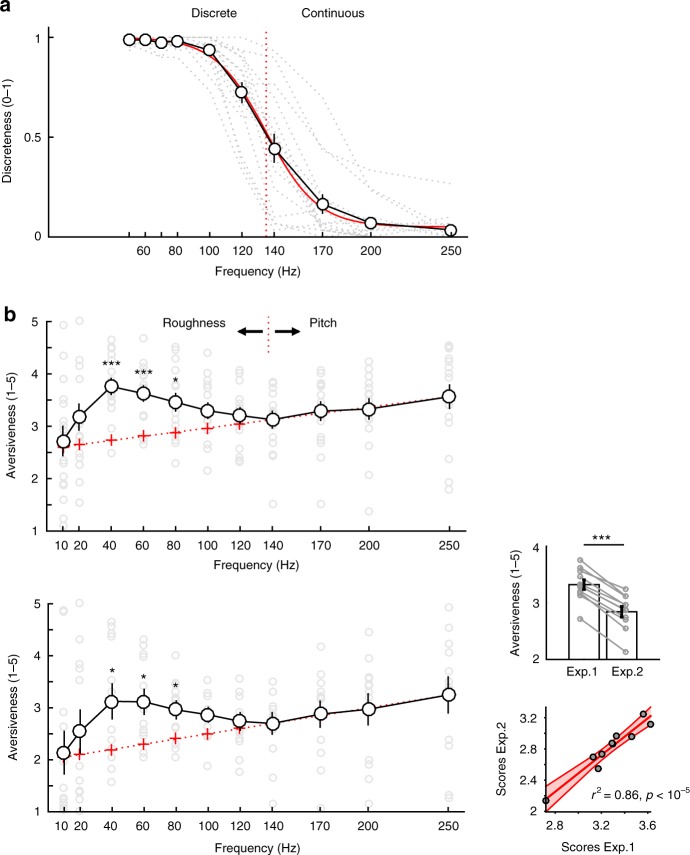
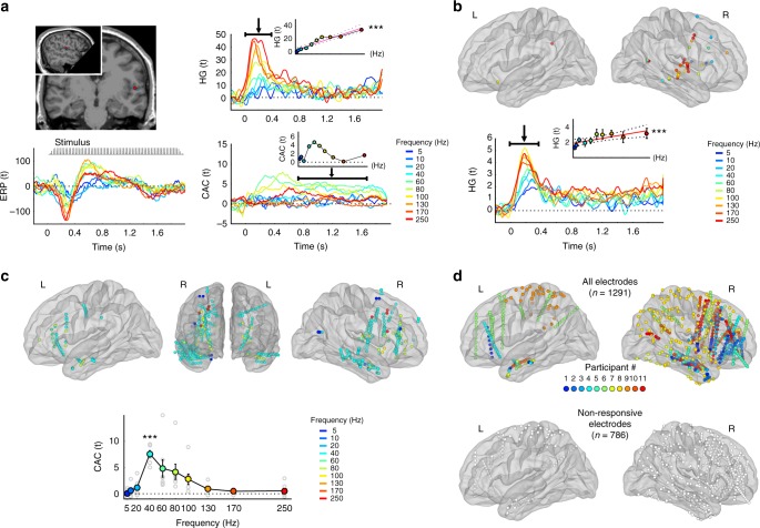
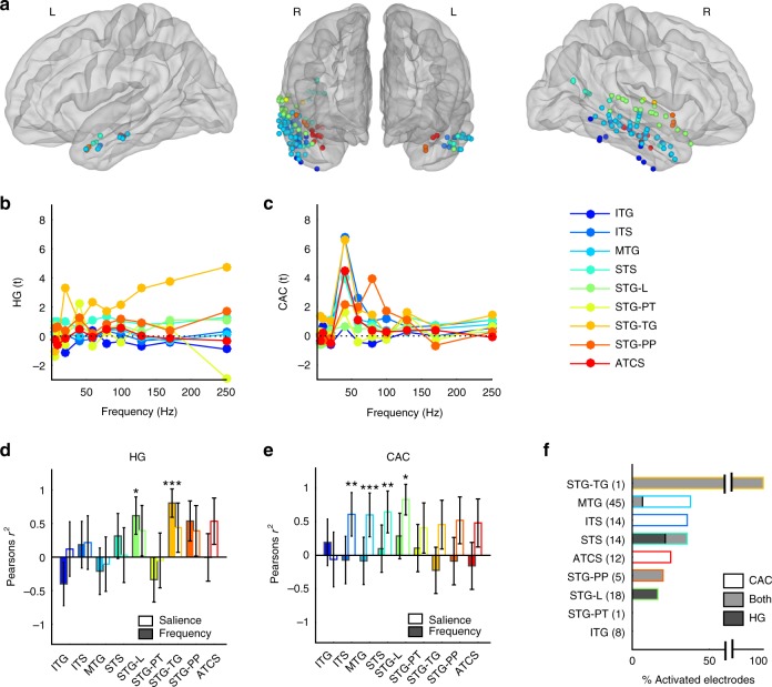
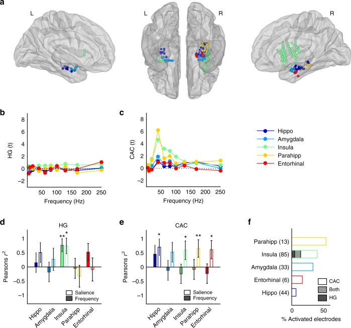
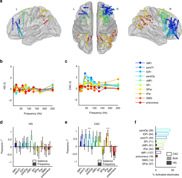
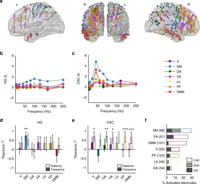
Being able to produce sounds that capture attention and elicit rapid reactions is the prime goal of communication. One strategy, exploited by alarm signals, consists in emitting fast but perceptible amplitude modulations in the roughness range (30-150 Hz). Here, we investigate the perceptual and neural mechanisms underlying aversion to such temporally salient sounds. By measuring subjective aversion to repetitive acoustic transients, we identify a nonlinear pattern of aversion restricted to the roughness range. Using human intracranial recordings, we show that rough sounds do not merely affect local auditory processes but instead synchronise large-scale, supramodal, salience-related networks in a steady-state, sustained manner. Rough sounds synchronise activity throughout superior temporal regions, subcortical and cortical limbic areas, and the frontal cortex, a network classically involved in aversion processing. This pattern correlates with subjective aversion in all these regions, consistent with the hypothesis that roughness enhances auditory aversion through spreading of neural synchronisation.

Fig. 1

Temporal perceptual transition and subjective assessment of temporal salience. a Temporal discretisation limit experiment (Experiment 1). Averaged subjective reports of discreteness (1–discrete, 0–continuous) averaged across participants indicate that subjective percept switches from discrete to continuous around 130 Hz (red dotted line: 50% discreteness ratings), which roughly corresponds to the upper limit of the roughness acoustic attribute. The continuous red curve represents the sigmoidal fit to the average across participants. Dotted light grey lines correspond to individual data. b Temporal salience experiments. Top panel: Experiment 2a. Averaged subjective aversion (reported on a 1–5 scale) follows a nonlinear pattern. Above the discretisation limit (>130 Hz, i.e., in the pitch range), aversion is linearly proportional to the frequency (energy) of the stimulus. Below this limit, in the roughness range, subjective aversion follows a nonlinear profile and is maximal at 40 Hz. Divergence from linearity in the roughness range is measured as the difference with aversion values predicted by a linear extrapolation of averaged aversion values measured above the discretisation limit. Light grey circles correspond to individual data Bottom panel: Experiment 2b: independent replication of Experiment 2a using the same stimuli at lower intensity (50 dB SPL) in n = 12 additional participants. Upper right inset: Main effect of sound intensity between Experiments 2a and 2b. Grey data points correspond to stimuli frequencies. Lower right inset: correlation plot between averaged ratings at each frequency in Experiment 2a and 2b. Error bars indicate SEM. ** and *** indicate significant p-values at 0.01 and 0.001, FDR corrected

Fig. 2

HG and CAC spatial response patterns differ across stimulation frequencies. a Neural responses to click trains in a representative electrode situated in the right primary auditory cortex (Heschl’s Gyrus) of patient S1. Lower left plot: time course of unfiltered event-related responses to the stimuli expressed in t-values relative to baseline. Responses are aligned with an exemplar of a stimulus (here a 40 Hz click train). Upper right plot: time course of high-gamma [HG, 70–200 Hz] amplitude in response to the stimulus, expressed in t-values relative to baseline, as a function of click train frequency (ranging from 5 Hz, blue to 250 Hz, red). HG onset [0–0.4 s] response is linearly proportional to the rate of the stimulus (upper inset). Lower right plot: magnitude squared stimulus-brain coherence (cerebro-acoustic coherence, CAC, expressed in t-values relative to baseline). CAC shows a sustained pattern through the duration of the stimulus that varies nonlinearly as a function of the stimulus rate and is prominent in the roughness range (40–100 Hz; lower inset). b–d Neural responses to click trains across all eleven patients. b Upper panel: spatial location of electrodes exhibiting significant HG onset responses to sounds. Colours represent the stimulation frequency at which HG response is maximal. Lower plot: time course of HG [70–200 Hz] responses averaged across these electrodes, expressed in t-values relative to baseline, as a function of stimulus frequency. HG amplitude at the response onset [0–400 ms] is linearly proportional to the rate of the stimulus (inset). c Electrodes showing sustained, significant stimulus-brain coherence (CAC) are spatially located in widespread cerebral areas. Colours represent the stimulation frequency at which CAC is maximal. Lower plot: CAC as a function of stimulus rate. Light grey circles correspond to individual data. d. Top panels: spatial location of all electrodes, colour-coded as a function of participant number. Lower panel: spatial location of electrodes that did not show any significant HG or CAC response. Error bars indicate SEM. Asterisks in panels a and b indicate significant correlation with stimulus frequency: *** indicates significant p-values at 0.001

Fig. 3

HG and CAC response patterns in anatomically defined sub-regions of the temporal lobe. a Anatomical and functional categorisation of electrodes in the temporal lobes, based on the Destrieux anatomical parcellation. b HG responses in onset [0–0.4 s] window (expressed in t-values relative to the baseline) averaged within regions and across participants at each stimulus frequency. c Same as in b. for CAC in late [0.8–1.8 s] window. d Pearson’s correlation value (r²) between onset HG responses and stimulus frequency (coloured filled bars) and salience (empty bars). Error bars indicate SE of the correlation. e Same as in (d) for CAC. f Proportion of activated electrodes exhibiting significant HG onset response (dark shading), sustained CAC (no shading) or both (grey shading) in each network. Numbers on the y-axis indicate the number of electrodes located in each regions. *, ** and *** indicate significant (corrected) p-values at 0.05, 0.01 and 0.001, respectively. ITG Inferior Temporal Gyrus, ITS Inferior Temporal Sulcus, MTG Middle Temporal Gyrus, STS Superior Temporal Sulcus, STG-L Superior Temporal Gyrus-Lateral, STG-PT Planum Temporale, STG-TG Transverse Gyrus, STG-PP Planum Polare, ATCS Anterior Transverse Collateral Sulcus

Fig. 4

HG and CAC response patterns in subcortical and limbic regions. a Anatomical and functional categorisation of electrodes in subcortical nuclei and limbic regions, based on the Desikan-Killiani anatomical parcellation. Left: left hemisphere, medial view. Centre: ventral view. Right: right hemisphere, medial view. b HG responses (expressed in t-values relative to the baseline) averaged within regions and across participants at each stimulus frequency. c Same as in b. for CAC. d Pearson correlation value (r²) between onset HG responses and stimulus frequency (colour-filled bars) and salience (empty bars). Error bars indicate SE of the correlation. e Same as in (d) for CAC. f Proportion of activated electrodes exhibiting significant HG onset response (dark shading), sustained CAC (no shading) or both (grey shading) in each region. Numbers on the y-axis indicate the number of electrodes located in each region. *, ** indicate significant (corrected) p-values at 0.05, 0.01, respectively. Hippo Hippocampus, Parahipp Parahippocampal Gyrus

Fig. 5

HG and CAC response patterns in frontal and parietal sub-regions. a Anatomical and functional categorisation of electrodes in frontal and parietal lobes, based on the Desikan-Killiani anatomical parcellation. b HG responses (expressed in t-values relative to the baseline) averaged within regions and across participants at each stimulus frequency. c Same as in (b) for CAC. d Pearson’s correlation value (r²) between onset HG responses and stimulus frequency (colour-filled bars) and salience (empty bars). Error bars indicate SE of the correlation. e Same as in (d) for CAC. f Proportion of activated electrodes exhibiting significant HG onset response (dark shading), sustained CAC (no shading) or both (grey shading) in each network. Numbers on the y-axis indicate the number of electrodes located in each region. *, ** indicate significant (corrected) p-values at 0.05, 0.01, respectively. rMFr rostral Middle Frontal, parsTr Pars Triangularis, iOFr inferior Orbito-Frontal, parsOp Pars Opercularis, cMFr Caudal Middle Frontal, SFr Superior Frontal, SPar Superior Parietal, iPar inferior Parietal, SMG Supra-Marginal Gyrus

Fig. 6

HG and CAC response patterns in functional connectivity networks. a Anatomical and functional categorisation of electrodes based on functional connectivity networks: sensori-motor (SM); limbic (Lb), default mode (DMN), ventral attention (DA), fronto-parietal (FP) and dorsal attention (DA). b HG responses (expressed in t-values relative to the baseline) averaged within regions and across participants at each stimulus frequency. c Same as in (b) for CAC. d Pearson’s correlation value (r²) between onset HG responses and stimulus frequency (colour-filled bars) or salience (empty bars). Error bars indicate SE of the correlation. e Same as in (d) for CAC. f Proportion of activated electrodes exhibiting significant HG onset responses (dark shading), sustained CAC (no shading) or both (grey shading) in each network. Numbers in parentheses on the y-axis indicate the overall number of electrodes located in each network. *, ** and *** indicate significant (corrected) p-values at 0.05, 0.01 and 0.001, respectively

References

1. Besser GM. Some physiological characteristics of auditory flutter fusion in man. Nature. 1967;214:17–19. doi: 10.1038/214017a0. - DOI - PubMed
1. Krumbholz K, Patterson RD, Pressnitzer D. The lower limit of pitch as determined by rate discrimination. J. Acoust. Soc. Am. 2000;108:1170–1180. doi: 10.1121/1.1287843. - DOI - PubMed
1. Fastl, H. & Zwicker, E. in Psychoacoustics. Facts and Models Vol. 22 111–148 (Springer-Verlag, Berlin, Heidelberg, 2007).
1. Terhardt, E. On the perception of periodic sound fluctuations (roughness). Acta Acust. united Ac. 30, 201–213 (1974).
1. von Helmholtz H. On the Sensations of Tone as a Physiological Basis for the Theory of Music. New York, NY: Dover; 1863.
Publication types