. 2019 Aug 23;10(1):3832.
doi: 10.1038/s41467-019-11736-2.

Integration of cortical population signals for visual perception

Affiliations

Integration of cortical population signals for visual perception

Ariana R Andrei et al. Nat Commun. .

Abstract

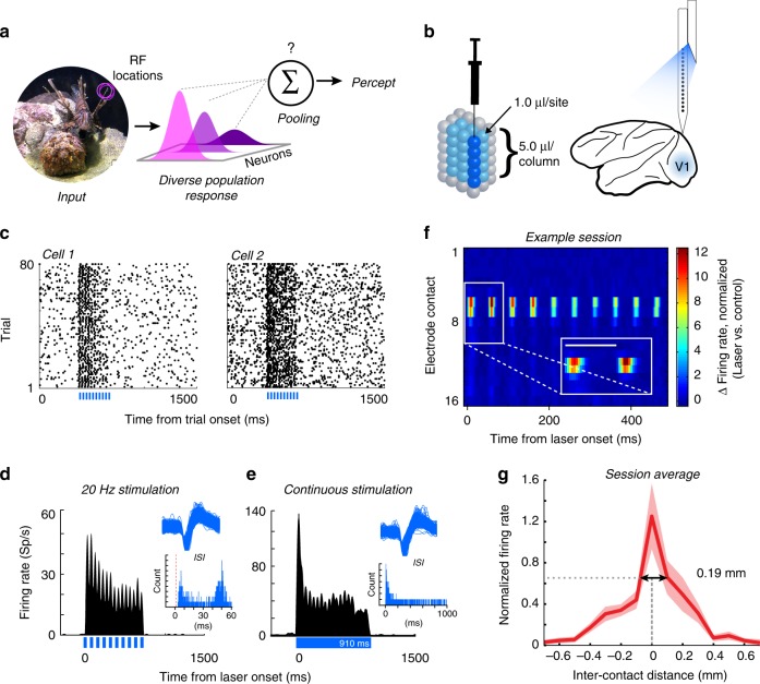
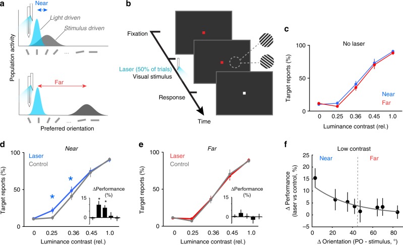
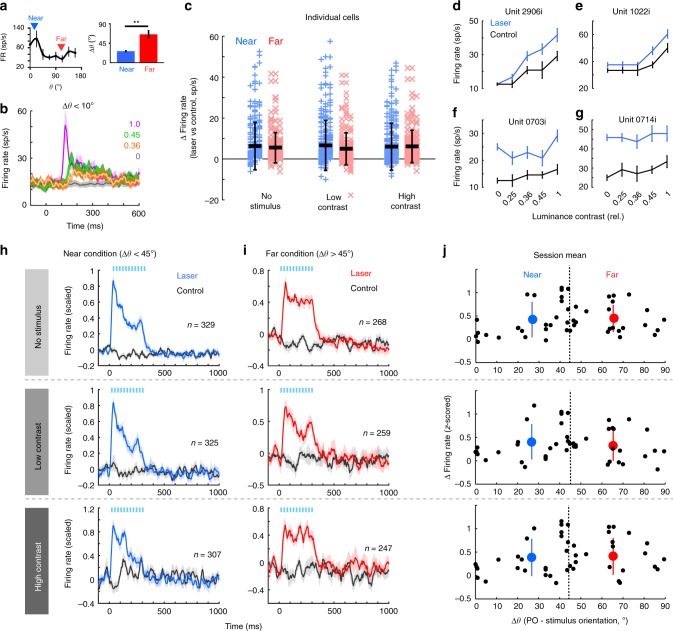
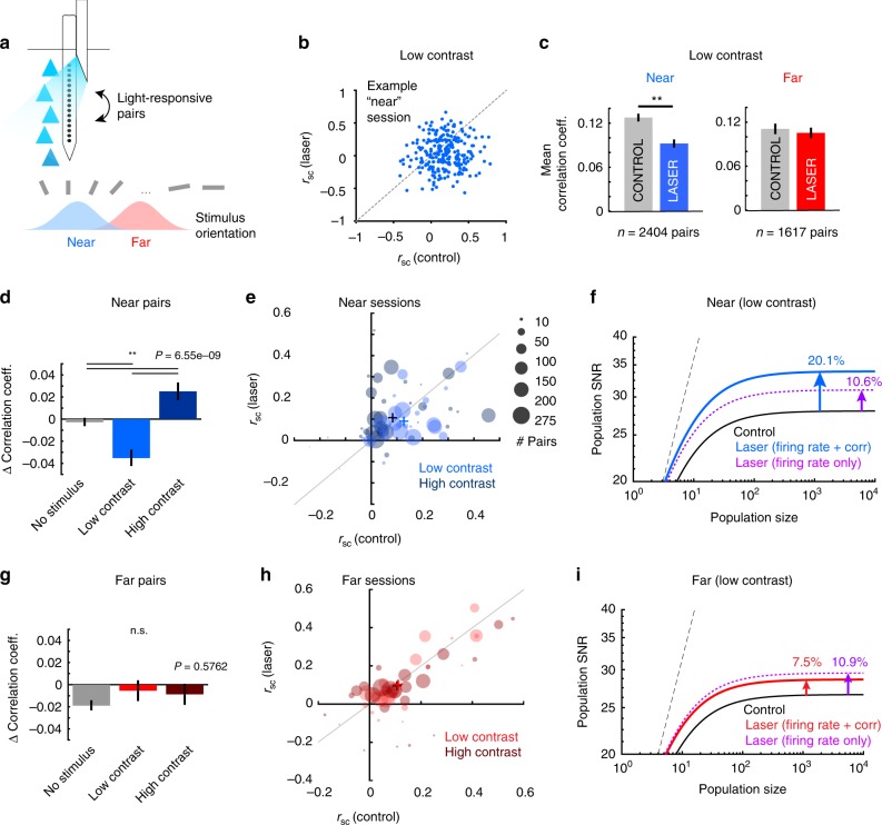
Visual stimuli evoke heterogeneous responses across nearby neural populations. These signals must be locally integrated to contribute to perception, but the principles underlying this process are unknown. Here, we exploit the systematic organization of orientation preference in macaque primary visual cortex (V1) and perform causal manipulations to examine the limits of signal integration. Optogenetic stimulation and visual stimuli are used to simultaneously drive two neural populations with overlapping receptive fields. We report that optogenetic stimulation raises firing rates uniformly across conditions, but improves the detection of visual stimuli only when activating cells that are preferentially-tuned to the visual stimulus. Further, we show that changes in correlated variability are exclusively present when the optogenetically and visually-activated populations are functionally-proximal, suggesting that correlation changes represent a hallmark of signal integration. Our results demonstrate that information from functionally-proximal neurons is pooled for perception, but functionally-distal signals remain independent.


Conflict of interest statement

The authors declare no competing interests.

Figures

Fig. 1
Fig. 1
Optogenetic targeting of localized neural subpopulations. a Sensory stimuli activate populations of diversely tuned neurons, whose activity is integrated according to unknown pooling rules to generate sensory percepts. b Virus injections and recordings were aligned with a custom grid. We injected 1.0 µl of virus in V1 at five cortical depths in a columnar fashion. Electrophysiological recordings were performed using laminar electrodes tightly coupled to a fiber optic for light delivery. c Raster plots from two example V1 neurons showing increased activity in response to pulsed light stimulation (laser timing shown in blue at the bottom of each plot), while the monkey fixated on a central point on a monitor. d, e To confirm the absence of optical artifacts, we compared the waveforms and firing rates of a sample of neurons (one example neuron shown) during pulsed (d) and continuous (e) laser stimulation. Upper insets show the distinct action potential waveforms recorded in each respective experiment. Lower insets show the interspike intervals (ISIs) in each stimulation condition. Vertical red dashed line denotes the 1 ms refractory period. Optical artifacts, when present, occur only at the onset and offset of optical stimulation and do not exhibit typical action potential waveform shapes. During pulsed stimulation (d, lower inset) the responses are distributed around the duration of each laser cycle period, without an intermediate peak at 10 ms corresponding to offset (width) of each individual laser pulse. Similarly during continuous stimulation (e, lower inset) there is no second peak that would correspond with laser offset. f Distribution of optically induced activity across electrode contacts for one example session. Inter-contact spacing is 100 µm (most superficial channel is labeled “1”). Inset shows blow up of the first two laser pulses (scale bar represents 50 ms). g Spatial spread of laser activation. Normalized firing rates were aligned with the channel showing the largest change in laser-induced activity, interpolating for distances between channels, and averaged across sessions. Negative inter-contact distances represent channels above (closer to the surface of the brain) the reference contact. Dashed lines and arrows show the spatial spread of laser activity at full width at half maximum. Error represents s.e.m.
Fig. 2
Fig. 2
Stimulus detection performance increases when the stimulated neural populations are nearby. a Cartoon showing how two neural populations can be simultaneously activated using light and visual stimulation. The functional distance between the two populations is controlled by changing the orientation of the visual stimulus to be “near” (upper) or “far” (lower) from the preferred orientation of the light-driven population. b Detection task design. Following a fixation period, oriented gratings are presented at four different contrasts. Half of trials contain no visual stimulus, and half of the trials are paired with optical stimulation. All contrasts and orientations are randomly interleaved. Monkeys are cued to report the presence or absence of a stimulus. c In the control (no laser) condition, detection performance for “near” and “far” stimulus orientations is similar for all contrast levels (P > 0.50 all contrasts, Wilcoxon signed rank tests). Error bars show s.e.m. d, e Percent target reports across sessions. Optogenetic stimulation-induced change in behavioral performance when the neural population is exposed to the “near” (d) and “far” stimulus (e). Optogenetic stimulation improves the detection of the two lowest contrast stimuli in the “near” condition (*P = 0.0025, Kruskal–Wallis test, df = 4, Chi-squared value = 16.43, post hoc Wilcoxon signed rank test), but had no impact in the “far” condition (e). Error bars show s.e.m. across sessions. f The light-induced enhancement in behavioral performance decays as the orientation difference between the two subpopulations increases. Black dots represent the mean change in target reports (laser vs. control) across sessions according to the orientation difference between the visual stimulus and the preferred orientation of the light-activated population (Sessions were grouped into 10° increments. Vertical dashed line shows the division between “near” and “far” categories. Fit is exponential. Error bars show s.e.m.
Fig. 3
Fig. 3
Light-evoked activity is uniform across stimulus orientations and contrasts. a, left Example orientation tuning curve for one neuron. Arrowheads represent the orientation of the “near” (blue) and “far” (red) stimuli presented in that session. a, right Mean difference between the neural population preferred orientation and stimulus orientation for “near” (blue) and “far” (red) conditions. **P = 2.8E-8, Wilcoxon rank sum test. Error shows s.e.m. b Mean firing rate of laser-responsive population on control trials, when the visual stimulus was within 10° of the preferred orientation of the neurons (n = 21). Colored lines represent different contrasts. Error bars show s.e.m. Firing rate change associated with laser for individual units in “near” (blue) and “far” (red) conditions (first 300 ms following light/stimulus onset). Thick horizontal bars represent the mean. Error bars represent the s.d. No group is significantly different from another (P = 0.10, one-way ANOVA, df = 5, F-statistic = 1.86). dg Contrast response functions for four example, light-responsive neurons (firing rates from 60–300 ms after stimulus onset). Error shows s.e.m. h, i Population mean firing rate (±s.e.m.) for all laser-responsive units recorded in “near” (h) and “far” (i) conditions. Rows correspond to contrast conditions. j Mean firing rate change per session across contrast conditions (rows). Black circles represent the mean firing rate changes across all simultaneously recorded light-responsive cells. Dashed vertical line shows the cutoff between “near” and “far” conditions. Large colored circles represent the mean change in firing rate across all “near” (blue) and “far” (red) sessions. Error bars show the standard deviation. The differences in laser-evoked firing rates are not statistically significant across stimulus contrast conditions (P = 0.35, Kruskal–Wallis test)
Fig. 4
Fig. 4
Optogenetic stimulation alters noise correlations and network performance in the “near” condition. a Noise correlations between light-responsive pairs along laminar electrode were measured across stimulus conditions. b Changes in noise correlations (“rsc”) for one example “near” condition session, during low contrast stimulus presentation. Each point represents correlation coefficients for one pair of laser-responsive cells in control and laser trials. c Population mean noise correlations for laser-responsive cell pairs during control (gray bars) and laser trials (colored bars) for “near” (left panel, blue) and “far” (right panel, red) conditions during low contrast presentation. (**Near sessions: P = 2.85e-6, Wilcoxon signed rank test, z-statistic = −4.68. Far sessions: P = 0.25, Wilcoxon signed rank test, z-statistic = −1.14). Error bars represent s.e.m. d, g Mean change in noise correlations following optogenetic stimulation for “near” (d) and “far” (g) across all stimulus conditions. Kruskal–Wallis test. Error bars are s.e.m. e, h Mean change in noise correlations for individual “near” (e) and “far” (h) sessions, at low (light circles) and high (dark circles) contrasts. Plus signs indicate cross session pair mean in each condition. Area of circle is proportional to the number of pairs from each session. f, i Impact of noise correlation changes on population SNR. Plots show SNR for hypothetical populations of increasing size for “near” (f) and “far” (i) subpopulations during presentation of low contrast stimuli. Solid lines show the SNR values during the control (black), and laser conditions for “near” (blue, f) and “far” (red, i) activated populations. Dotted magenta lines represent the change in SNR attributable to light-induced increase in firing rates alone, if noise correlations remain unchanged. Dashed black line represents the hypothetical SNR if there was no correlated noise
Fig. 5
Fig. 5
Functional distance-weighted pooling correlates best with detection performance. a Basic model of sensory detection relying on pooling signals across neural populations. Stimulus detection requires the pooled signals from V1 (colors represent different tuning preferences) to exceed a critical SNR threshold. b Two possible models of signal pooling. Upper A uniform pooling rule in which the total SNR is based equally on the sum of the visually driven response (gray, filled distribution) and the laser-driven response (colored, unfilled distributions), regardless of tuning difference (colors). Lower A distance-weighted pooling rule, in which the contribution of the laser-driven population is weighted by its orientation-difference from the visually driven population. The weight (w) is a simple exponential decay (see main text). c Total SNR predicted by uniform pooling for low contrast stimuli. The laser-driven neuronal activation in both the “near” (blue) and “far” (red) conditions substantially increases total SNR above the control condition (gray). Dashed black horizontal line estimates the global SNR threshold based on the control condition. d Total SNR predicted by functional distance (difference in orientation) weighted pooling for low contrast stimuli. Only the laser-driven neuronal activation in the “near” condition (blue) increases the total SNR substantially above the control condition, matching well with the laser-induced change in behavior (e). e Behavioral detection performance for low contrast stimuli in the absence of laser stimulation (gray), and with laser stimulation in the “near” (blue), and “far” (red) conditions. Error bars represent s.e.m. across sessions. Dashed black horizontal line estimates the detection threshold based on the control condition. f Percent change in total SNR following laser stimulation using functional distance-weighted pooling, calculated as a function of the orientation difference between the laser and visually driven populations. SNRs were estimated from bootstrapped data sampled every 10 sessions (ordered by Δθ), sliding every five sessions. Thick black line shows an exponential fit to the data points. Flanking thin black lines show the 95% confidence intervals for the fit. g Change in behavioral performance (laser vs. control), averaged across the same sessions used in f. Thick black bar shows an exponential fit to the data. Flanking thin black lines show the 95% confidence intervals for the fit

References

    1. Leopold DA. Primary visual cortex: awareness and blindsight. Annu. Rev. Neurosci. 2012;35:91–109. doi: 10.1146/annurev-neuro-062111-150356. - DOI - PMC - PubMed
    1. Tong F. Primary visual cortex and visual awareness. Nat. Rev. Neurosci. 2003;4:219–229. doi: 10.1038/nrn1055. - DOI - PubMed
    1. Nienborg H, Cumming BG. Macaque V2 neurons, but not V1 neurons, show choice-related activity. J. Neurosci. 2006;26:9567–9578. doi: 10.1523/JNEUROSCI.2256-06.2006. - DOI - PMC - PubMed
    1. Hubel DH, Wiesel TN. Receptive fields and functional architecture of monkey striate cortex. J. Physiol. 1968;195:215–243. doi: 10.1113/jphysiol.1968.sp008455. - DOI - PMC - PubMed
    1. Ringach DL, Shapley RM, Hawken MJ. Orientation selectivity in macaque V1: diversity and laminar dependence. J. Neurosci. 2002;22:5639–5651. doi: 10.1523/JNEUROSCI.22-13-05639.2002. - DOI - PMC - PubMed

Publication types