Characterizing micro-to-millisecond chemical exchange in nucleic acids using off-resonance R1ρ relaxation dispersion

Abstract

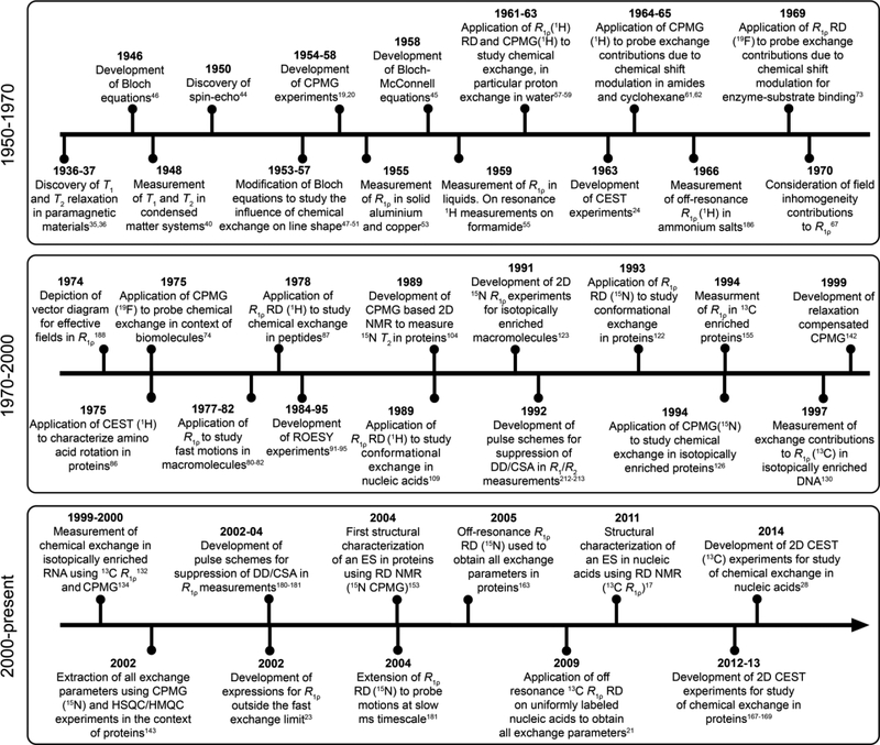
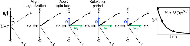
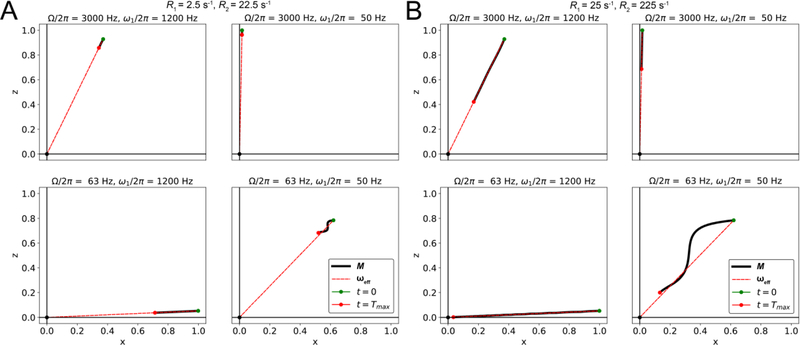
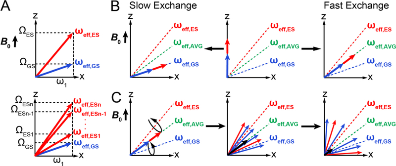
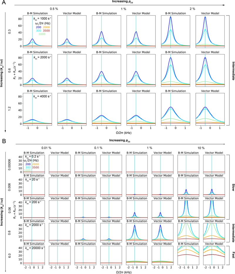
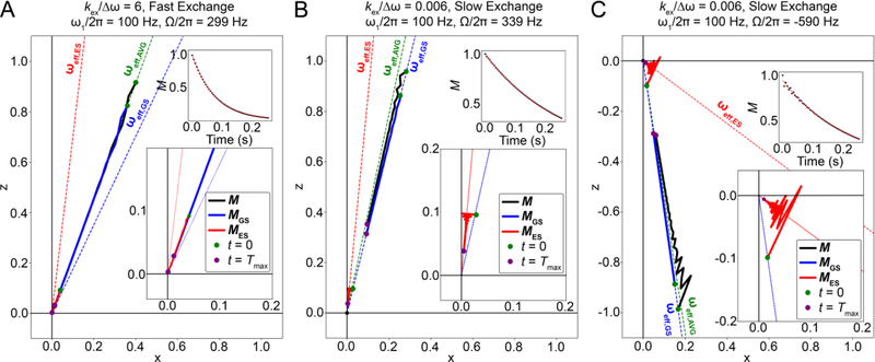
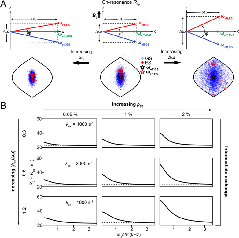
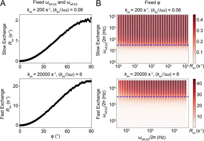
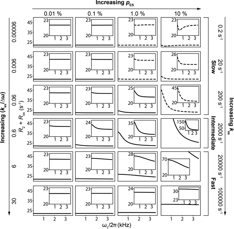
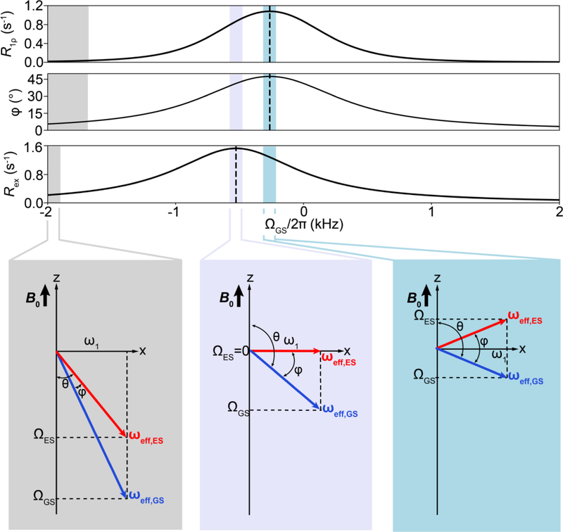
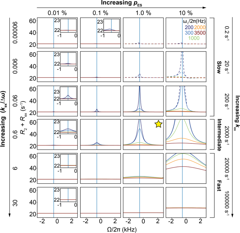
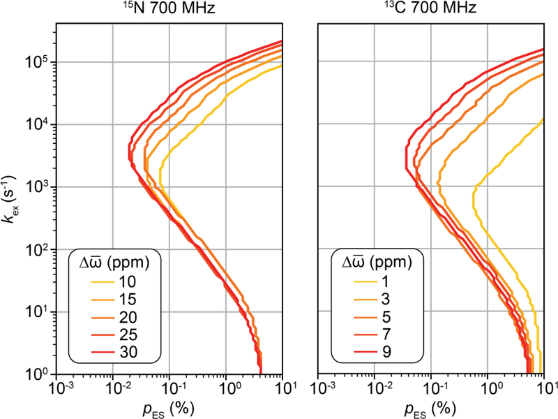
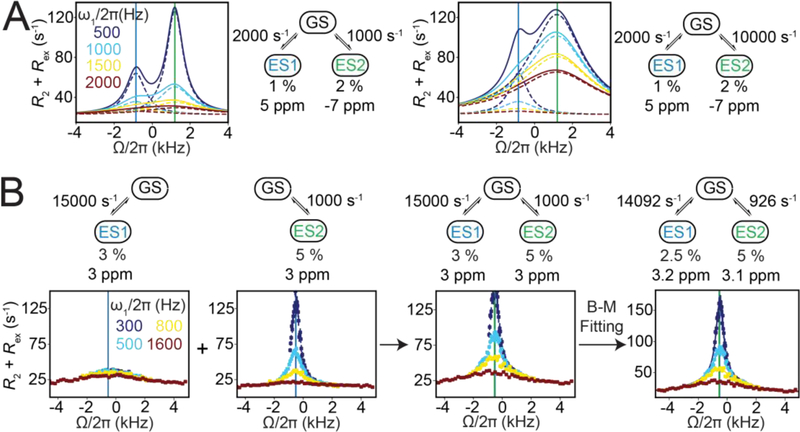
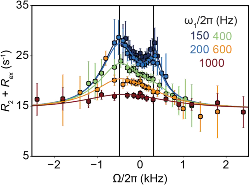
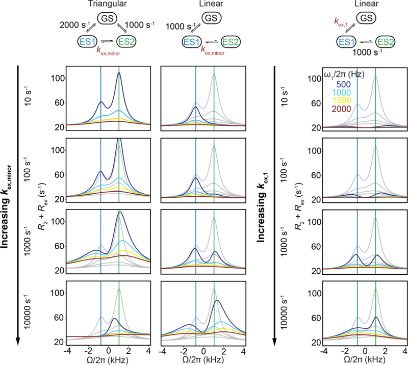
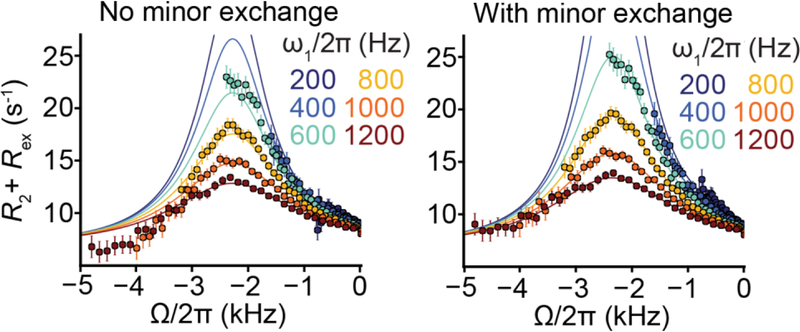
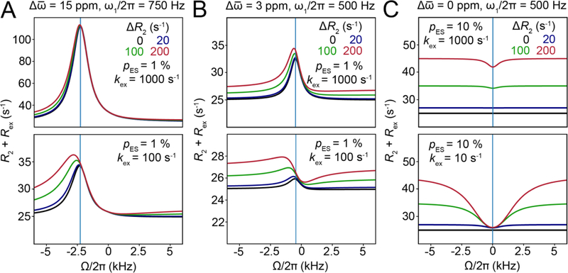
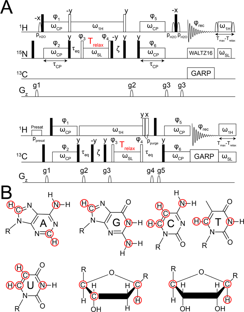
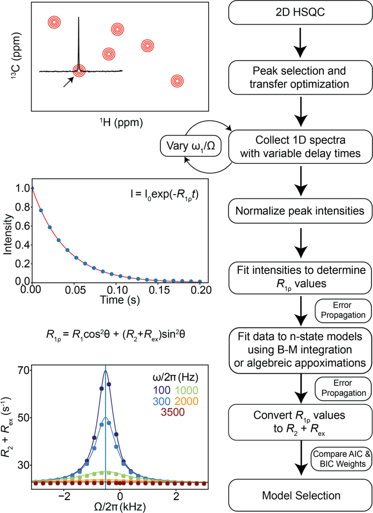
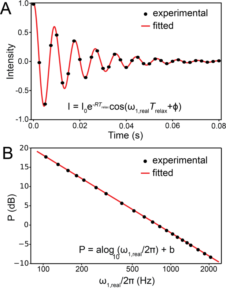
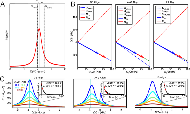
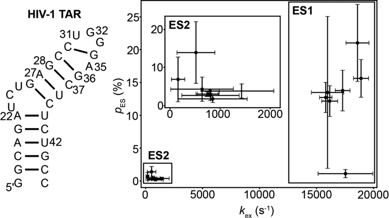
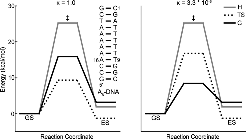
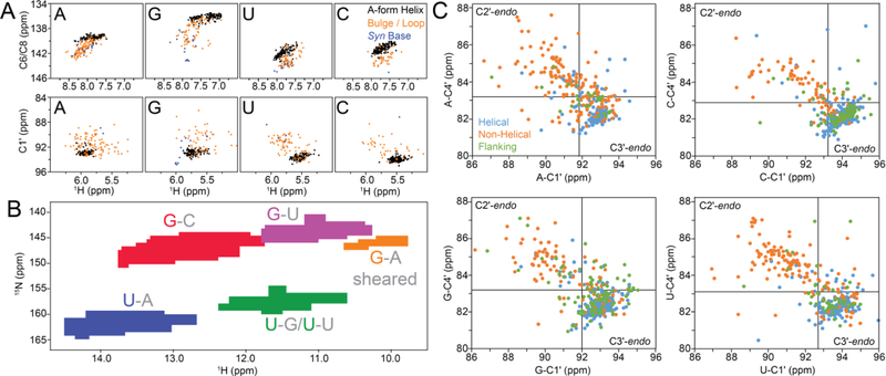
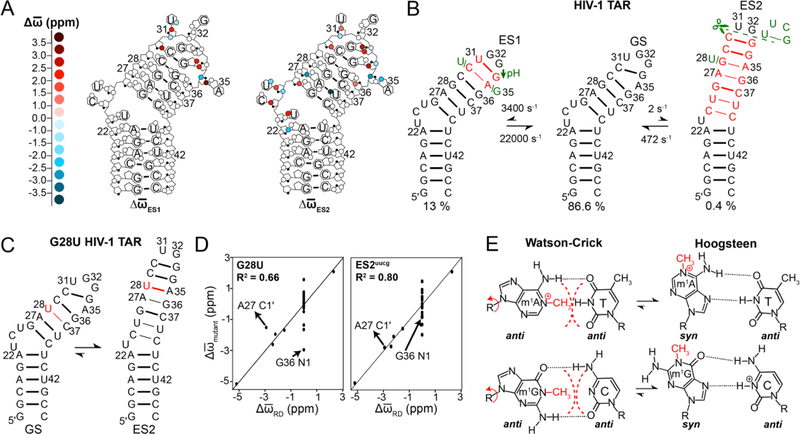
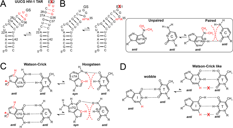
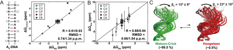
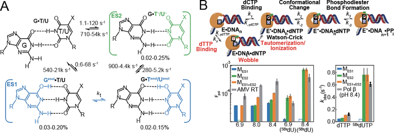
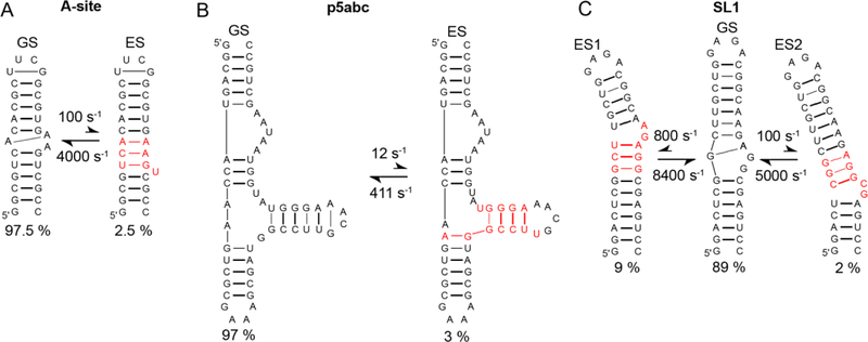
This review describes off-resonance R_1ρ relaxation dispersion NMR methods for characterizing microsecond-to-millisecond chemical exchange in uniformly ¹³C/¹⁵N labeled nucleic acids in solution. The review opens with a historical account of key developments that formed the basis for modern R_1ρ techniques used to study chemical exchange in biomolecules. A vector model is then used to describe the R_1ρ relaxation dispersion experiment, and how the exchange contribution to relaxation varies with the amplitude and frequency offset of an applied spin-locking field, as well as the population, exchange rate, and differences in chemical shifts of two exchanging species. Mathematical treatment of chemical exchange based on the Bloch-McConnell equations is then presented and used to examine relaxation dispersion profiles for more complex exchange scenarios including three-state exchange. Pulse sequences that employ selective Hartmann-Hahn cross-polarization transfers to excite individual ¹³C or ¹⁵N spins are then described for measuring off-resonance R_1ρ(¹³C) and R_1ρ(¹⁵N) in uniformly ¹³C/¹⁵N labeled DNA and RNA samples prepared using commercially available ¹³C/¹⁵N labeled nucleotide triphosphates. Approaches for analyzing R_1ρ data measured at a single static magnetic field to extract a full set of exchange parameters are then presented that rely on numerical integration of the Bloch-McConnell equations or the use of algebraic expressions. Methods for determining structures of nucleic acid excited states are then reviewed that rely on mutations and chemical modifications to bias conformational equilibria, as well as structure-based approaches to calculate chemical shifts. Applications of the methodology to the study of DNA and RNA conformational dynamics are reviewed and the biological significance of the exchange processes is briefly discussed.

Keywords: Chemical exchange; Hoogsteen; Nucleic acid dynamics; R(1ρ) relaxation dispersion; Tautomers.

Figure 1.

Time diagram showing key developments in RD NMR techniques for characterizing chemical exchange in biomolecules with emphasis placed on R_1ρ studies and their application to nucleic acids.

Figure 2.

Historical progression of the development of R_1ρ RD techniques for applications to nucleic acids. A) The on-resonance R_1ρ(¹H) RD profile measured for formamide by Solomon et al.[55] was the first reported measurement of R_1ρ in liquids. Reproduced with permission from Bibliotheque nationale de France (BNF).B) The chair-chair inter-conversion in cyclohexane was one of the earliest conformational transitions characterized by RD methods[62, 63].C) R_1ρ(¹⁹F)measurements on N-trifluoroacetyl phenylalanine in exchange between free and enzyme-bound states by Sykes et al.[73] constituted the first application of R_1ρ RD in the context of biological macromolecules. D) Some of the earliest applications of R_1ρ in studies of conformational exchange in biomolecules targeted ¹H nuclei (red circles) in nucleic acid duplexes in the early 1990s[–111]. E) On-resonance R_1ρ(¹⁵N) RD profile for backbone amide ¹⁵N of C38 in bovine pancreatic trypsin inhibitor was one of the first reported characterizations of conformational exchange in isotopically labeled proteins using R_1ρ[122]. Reprinted by permission from [122]. F) Secondary structure transition in U6RNA involving flipping out of a bulge nucleotide; this was one of the first validated models for ESs in nucleic acids[135]. G) First structure of an ES by Kay et al.[153] for a folding intermediate of the G48V mutant of the Fyn SH3 domain obtained using chemical shifts measured using CPMG RD and structurebased chemical shift calculations. Reprinted by permission from [153]. H) Expressions for R_1ρ outside the fast exchange limit by Palmer et al.[23] allowed extensions of the R_1ρ method by demonstrating the feasibility of extracting all exchange parameters at a single magnetic field. RD profiles were shown to be centered at the ES chemical shift. Simulated off-resonance profiles (for p_ES = 0.048, k_ex = 1500 s⁻¹, Δω = 2400 rad s⁻¹, R_1,GS = R_1,ES = 1.5 s⁻¹, R_2,GS = R_2,ES = 11 s⁻¹ and ω₁/2π = 1000 Hz) are shown using the asymmetric population expression in Palmer et al.[23] (dotted line) and fast exchange expression (dashed line). The exact numerical solution is shown as a solid black line. Reproduced with permission from [23]. I) Off-resonance R_1ρ(¹⁵N) RD profile for the amide ¹⁵N of Q11 in a G48M mutant of the Fyn-SH3 domain; this was the first experimental measurement of off-resonance R_1ρ using low spin-lock amplitudes and selective excitation experiments[163]. This study also represented the first instance wherein a complete set of exchange parameters was extracted using R_1ρ measurements. Reprinted with permission from [163]. J) Excited state Hoogsteen BPs in duplex DNA were the first ESs to be structurally characterized in nucleic acids using R_1ρ RD.Rates and populations were obtained using off-resonance R_1ρ experiments as described by Al-Hashimi et al.[115].

Figure 3.

Thermodynamic and kinetic characteristics of a system undergoing two-state chemical exchange. A) Free energy diagram for two-state exchange. B) Time evolution of a molecule exchanging between a dominant GS and sparsely populated and short-lived ES. C) Distribution of τ_GS and τ_ES, the dwell times for the GS and ES.

Figure 4.

Chemical exchange under free precession. A) NMR spectra for a system undergoing two-state GS-ES chemical exchange simulated using the B-M equations. Columns correspond to different values of p_GS while rows correspond to different values of k_ex. Simulations were performed assuming $\Delta \overline{\omega }{\text{ (}}^{13}\text{C)}=3\text{\hspace{0.17em}ppm}$, γ(¹H)B₀/2π = 700 MHz and R_2,GS = R_2,ES = 10 s⁻¹. B) Magnetization of GS (blue) and ES (red) spins in the rotating frame of the GS at the slow exchange limit. Black arrows represent the passage of time while colored arrows represent exchange events. Dots surrounded by circles denote vectors perpendicular to the plane of the figure. C) GS-ES chemical exchange leads to dephasing with time of the bulk magnetization corresponding to the GS (black arrow). The black dot near the x-axis corresponds to the receiver phase. D) Exponential decay due to chemical exchange of the bulk GS magnetization along the x axis (M_GSx) as a function of time. E) The magnetization of the GS (blue) and ES (red) spins in the rotating frame of the population-weighted average (AVG) resonance in the fast exchange limit.

Figure 5.

The mono-exponential decay of magnetization due to chemical exchange under free precession conditions is a consequence of the exponential dwell time distributions of the GS and ES. (A and B) Normalized bulk x-magnetization M_GSx (black dots) of the GS as a function of time for a system undergoing GS-ES exchange, simulated using the vector model. An exponential fit to the magnetization is shown in red. Panel A is simulated assuming exponential probability distributions for the GS and ES dwell times (< τ_GS > = 0.33 s and < τ_ES > = 0.14 s), while panel B is simulated assuming that the ES and GS dwell times follow a standard normal distribution. Expressions for the probability distributions of τ_GS and τ_ES are given in the inset. Simulations assumed the following exchange parameters: $\Delta \overline{\omega }{\text{ (}}^{13}\text{C)}=3\text{\hspace{0.17em}ppm}$, γ(¹H)B₀/2π = 700 MHz, and R_1,GS= R_1,ES = R_2,GS = R_2,ES = 0 s⁻¹ for panels A and B.

Figure 6.

Line-width at half maximum (LW_1/2, units Hz) for the dominant GS resonance as a function of $\Delta \overline{\omega }$ for a system undergoing GS-ES exchange under free precession, simulated using the B-M equations (k_ex = 1500 in red and k_ex = 2750 in black). Simulations assumed the following exchange parameters: p_ES = 0.05, γ(¹H)B₀/2π = 700 MHz, R_1,GS= R_1,ES = R_2,GS = R_2,ES = 0.0 s⁻¹, while $\Delta \overline{\omega }{\text{ (}}^{13}\text{C)}$ was varied linearly between 0.1 and 40 ppm in 100 equally spaced increments. Solid lines denote (R₂+p_ESk_ex)/π while dotted lines denote a Δω value where (k_ex/Δω) ~ 0.2.

Figure 7.

Influence of the spin-locking field during an R_1ρ experiment in the absence of chemical exchange. A) In the lab frame (left), the spin-locking field B₁ (black arrow) can be decomposed into two fields $B_1^{+}$ and $B_1^{-}$ rotating in opposite directions (green and cyan arrows). The short black arrow represents the passage of time. A black dot surrounded by a circle represents a vector perpendicular to the plane of the figure. Black dots near the x-axes correspond to the receiver phase. ω_rf is the angular frequency of the spin-lock. Variation of the spin-locking field amplitude as a function of time is shown on the right. B) Evolution of $B_1^{+}$ and $B_1^{-}$ in the rotating frame of $B_1^{+}$. The static magnetic field is reduced to ΔB. C) Effective fields under on- and off-resonance conditions in the rotating frame of the spin-lock.

Figure 8.

Modulation of the effective field by variation of the spin-lock amplitude (ω₁) and offset frequency (Ω) in an R_1ρ experiment in the absence of chemical exchange. Influence of changing ω₁ (A) and Ω (B) on the effective field ω_eff in the rotating frame.

Figure 9.

Schematic representation of the R_1ρ experiment in the absence of chemical exchange. The equilibrium magnetization tilted along z′, the direction of ω_eff,OBS, is immediately spin-locked by the application of an RF field (green arrow), after which it decays exponentially due to relaxation with a rate constant R_1ρ. A cross within a circle denotes a vector perpendicular to the plane of the figure. All vector diagrams are in the rotating frame where the spin-locking field appears stationary.

Figure 10.

Time course of the evolution of normalized magnetization during an R_1ρ experiment in the absence of chemical exchange, as a function of the spin-lock amplitude ω₁, the offset Ω and the relaxation rates, simulated using the B-M equations. A) R₁ = 2.5 s⁻¹ and R₂ = 22.5 s⁻¹; B) R₁ = 25 s⁻¹ and R₂ = 225 s⁻¹. The time course for the position of the tip of the net magnetization vector M (with its base at the origin) is denoted as a solid black line, with green and red dots denoting the positions of the vector tip at the start and end (T_max = 0.015s) of the relaxation period, respectively. The effective field direction is denoted using a dashed red line.

Figure 11.

R_1ρ in the presence of chemical exchange. A) ω_eff,GS (blue) and ω_eff,ES (red) in the rotating frame where the spin-locking field ω₁ appears stationary, for two-state and n-state exchange. B) Alignment of the net magnetization at the start of an R_1ρ experiment for a system undergoing GS-ES exchange under fast and slow exchange regimes. C) Rotation of the magnetization of GS/ES spins around their respective effective fields leads to dephasing of the bulk magnetization along ω_eff,OBS during the R_1ρ experiment. Shown is a representative example under conditions of fast exchange.

Figure 12.

Comparison of off-resonance R_1ρ RD profiles as obtained from B-M simulations and the vector model, in the absence of relaxation, for a wide variety of exchange parameters. Rows correspond to variations in k_ex while columns correspond to variations in p_ES. Spin-lock amplitudes are color coded while solid vertical green lines correspond to an offset Ω = –Δω; $\Delta \overline{\omega }{(}^{13}\text{C)}=3\text{\hspace{0.17em}ppm}$, γ(¹H)B₀/2π = 700 MHz. 10,000 spins were used for the vector model simulations. The initial alignment of the magnetization for the B-M and vector simulations was performed as described in Section 6.1. In the vector model simulations, the magnetization of the GS and ES spins initially aligned along ω_eff,OBS was allowed to precess about ω_eff,GS and ω_eff,ES with angular velocities ω_eff,GS and ω_eff,ES, respectively. The dwell times of the spins in the GS and ES were sampled from exponential probability distributions as described in Section 3.1, following which they were allowed to exchange with each other, while retaining the same orientation of the magnetization in 3D space prior to exchange. The sum of the magnetization of all the spins is projected along ω_eff,OBS as a function of time to obtain R_1ρ, which is used to obtain R_ex, as described in Section 3.2 – 3.4.

Figure 13.

Time course of the evolution of the normalized GS, ES and net magnetization during an off-resonance R_1ρ experiment, simulated using the B-M equations. Time course for the positions of the tips of the GS, ES and net magnetization vectors (each with their base at the origin), denoted as solid blue, red and black lines respectively, with green dots in each case denoting the positions of the vector tips at the start of the relaxation period, and violet dots denoting their positions at the end of the relaxation period, respectively. Directions for the GS,ES and AVG effective fields are denoted using blue, red and green dashed lines, respectively. Also shown as insets are the variations of the normalized projections of the net magnetization along ω_eff,OBS (M) as a function of time (black dots), along an exponential fit of the same (red line). Simulations were performed using k_ex = 20000 s⁻¹ for panel A, k_ex = 20 s⁻¹ for panels B and C. The other parameters used for all simulations were p_ES = 0.1, $\Delta \overline{\omega }{(}^{13}\text{C)}=3\text{\hspace{0.17em}ppm}$, γ(¹H)B₀/2π = 700 MHz, R_1,GS = R_1,ES = 2.5 s⁻¹, R_2,GS = R_2,ES = 22.5 s⁻¹ and T_max = 0.25 s. The initial alignment of the magnetization for the B-M and vector simulations was achieved as described in Section 6.1.

Figure 14.

Dependence of on-resonance R_1ρ on exchange and spin-lock parameters.A) Δω and ω₁ modulate R_ex via changes in φ, the angle between ω_eff,GS and ω_eff,ES. Also shown are positions of the magnetization vectors corresponding to GS (blue circles) and ES (red circles) obtained using vector model simulations in the form of Sanson-Flamsteed projections[192]. ω_eff,GS and ω_eff,ES are indicated by black and red stars respectively. Simulations were performed with the following parameters - p_ES = 0.01, k_ex = 20,000 s⁻¹, $\Delta \overline{\omega }{(}^{13}\text{C)}=3\text{\hspace{0.17em}ppm}$, γ(¹H)B₀/2π = 700 MHz, ω₁/2π = 1000 Hz when on-resonance with the AVG state. Positions of the spins for a larger $\Delta \overline{\omega }{(}^{13}\text{C)}=10\text{\hspace{0.17em}ppm}$ (right) and ω₁/2π = 3000 Hz (left) are also shown. Simulations employed 10,000 spins with a relaxation delay of 0.012s.B) Variation of R₂ + R_ex with ω₁ under on-resonance conditions as a function of exchange parameters, as obtained using B-M simulations. Rows and columns correspond to the indicated values of k_ex and p_ES, respectively. Dashed line denotes the value of R₂. The other exchange parameters used were $\Delta \overline{\omega }{(}^{13}\text{C)}=3\text{\hspace{0.17em}ppm}$, γ(¹H)B₀/2π = 700 MHz, R_1,GS= R_1,ES = 2.5 s⁻¹ and R_2,GS = R_2,ES = 22.5 s⁻¹. The initial alignment of the magnetization during the B-M simulations was performed as described in Section 6.1.

Figure 15.

Vector model simulations to illustrate the dependence of R_ex on φ, ω_eff,GS and ω_eff,ES during an on-resonance R_1ρ experiment for a system undergoing two-state GS-ES exchange. A) Variation of R_ex with φ for a fixed ω_eff,GS and ω_eff,ES, under fast and slow exchange conditions. Simulations were performed using ω_eff,GS = 1000*2π rad s⁻¹ and ω_eff,ES = 1131*2π rad s⁻¹ when on-resonance with the GS under slow exchange conditions. ω_eff,GS = 1000*2π rad s⁻¹ and ω_eff,ES = 1128*2π rad s⁻¹ under fast exchange conditions while maintaining the AVG state onresonance by suitably adjusting the offset of the GS and ES. Similar trends are observed for alternative values of the precession frequencies (data not shown). B) Heat maps of R_ex as a function of ω_eff,GS and ω_eff,ES for a fixed φ under fast and slow exchange conditions. Horizontal dotted lines (blue) correspond to the condition ω_eff,ES = k_ex. Orientations of the effective fields were kept fixed at those corresponding to application of ω₁/2π = 1000 Hz on resonance. Similar trends are also observed for R_1ρ, and for both R_ex and R_1ρ under off-resonance conditions, as long as the magnetization decay is mono-exponential (data not shown). For panels A and B, simulations were performed using 10,000 spins with p_ES = 0.01, $\Delta \overline{\omega }{(}^{13}\text{C)}=3\text{\hspace{0.17em}ppm}$, γ(¹H)B₀/2π = 700 MHz, R_1,GS= R_1,ES = 0.0 s⁻¹, R_2,GS = R_2,ES = 0.0 s⁻¹. The relaxation delays used were 3 s and 0.6 s for k_ex = 200 and 20000 s⁻¹, respectively. For both panels, the initial alignment of magnetization and its projection to calculate R_ex, was performed as described in Section 6.1.

Figure 16.

Variation of R₂ + R_ex as a function of ω₁ under on-resonance conditions as a function of exchange parameters, obtained using B-M simulations. Rows and columns correspond to the indicated values of k_ex and p_ES respectively. Panels with dotted lines correspond to exchange scenarios where the decay of the magnetization is not mono-exponential. Other parameters were: $\Delta \overline{\omega }{(}^{13}\text{C)}=3\text{\hspace{0.17em}ppm}$, γ(¹H)B₀/2π = 700 MHz, R_1,GS = R_1,ES = 2.5 s ⁻¹ and R_2,GS = R_2,ES = 22.5 s⁻¹. The initial alignment of the magnetization was performed as described in Section 6.1.

Figure 17.

Variation of R_1ρ, φ and R_ex with Ω_GS during an off-resonance R_1ρ experiment under slow-exchange conditions with ω_eff,ES < k_ex. Representative diagrams showing ω_eff,GS (blue vector) and ω_eff,ES (red vector) at selected offsets are also shown. The exchange parameters used were: p_ES = 0.01, k_ex = 200 s⁻¹, $\Delta \overline{\omega }{(}^{13}\text{C)}=3\text{\hspace{0.17em}ppm}$, γ(¹H)B₀/2π = 700 MHz, R_1,GS= R_1,ES = 0.0 s⁻¹, R_2,GS = R_2,ES = 0.0 s⁻¹, ω₁/2π = 600 Hz along with a relaxation delay of 3.0 s. The initial alignment of the magnetization during the B-M simulation was performed as described in Section 6.1.

Figure 18.

Changes in R₂ + R_ex as a function of k_ex and p_ES for two-state exchange during an off-resonance R_1ρ experiment, simulated using the B-M equations. Horizontal comparisons show changes in k_ex while vertical comparisons show changes in p_ES. Spin-lock amplitudes are denoted using different colors. Solid gray vertical lines correspond to an offset of –Δω, while the yellow star denotes exchange parameters typical of Watson-Crick to Hoogsteen exchange in B-DNA[115]. Other exchange parameters used are: $\Delta \overline{\omega }{(}^{13}\text{C)}=3\text{\hspace{0.17em}ppm}$, γ(¹H)B₀/2π = 700 MHz, R_1,GS = R_1,ES = 2.5 s ⁻¹ and R_2,GS = R_2,ES =22.5 s⁻¹. The initial alignment of the magnetization was performed as described in Section 6.1.

Figure 19.

Variation of R₂ + R_ex with k_ex during an R_1ρ experiment when on-resonance with the ES (p_ES = 0.01, $\Delta \overline{\omega }{(}^{13}\text{C)}=3\text{\hspace{0.17em}ppm}$, γ(¹H)B₀/2π = 700 MHz, R_1,GS = R_1,ES = 2.5 s ⁻¹ and R_2,GS = R_2,ES =22.5 s⁻¹). Spin-lock amplitudes are color-coded. Vertical lines denote the indicated values of k_ex. The initial alignment of the magnetization during the B-M simulations was performed as described in Section 6.1.

Figure 20.

Representative experimental off-resonance R_1ρ RD profiles for two-state exchange under fast and intermediate exchange. The profiles were measured for U31-C1′ and C24-C1′ in HIV-1 TAR at 25 °C and 35 °C, respectively[166]. Spin-lock amplitudes are color-coded. Error bars represent experimental uncertainties determined by a Monte-Carlo scheme (Section 6.3). Solid lines denote global fits to the RD data using the B-M equations[166]. The initial alignment of the magnetization during the B-M fitting was performed as described in Section 6.1. Gray vertical lines correspond to the offset value when on resonance with the ES. Reproduced with permission from [166].

Figure 21.

Variation of R₂ + R_ex during off-resonance R_1ρ experiments, for a wide range of k_ex and p_ES values for two-state exchange, simulated using the B-M equations. Horizontal comparisons show changes in k_ex while vertical comparisons show changes in p_ES. Different spin-lock amplitudes are denoted by colors. Dotted lines correspond to cases where the decay of the magnetization is not mono-exponential. Solid gray vertical lines correspond to an offset of –Δω, while the yellow star denotes a typical Watson-Crick to Hoogsteen exchange scenario in DNA[115]. Simulations assumed the following parameters: $\Delta \overline{\omega }{(}^{13}\text{C)}=3\text{\hspace{0.17em}ppm}$, γ(¹H)B₀/2π = 700 MHz, R_1,GS = R_1,ES = 2.5 s ⁻¹ and R_2,GS = R_2,ES = = 22.5 s⁻¹. The initial alignment of the magnetization was performed as described in Section 6.1.

Figure 22.

Exploring the limits of the sensitivity for off-resonance R_1ρ experiments using B-M simulations for R_1ρ(¹⁵N)(left) and R_1ρ(¹³C) (right), at γ(¹H)B₀/2π = 700 MHz. For each $\Delta \overline{\omega }$ value, detectability of R_1ρ was assessed for 10,000 (p_ES, k_ex) combinations. 100 p_ES values ranging between 0.005 % to 20 % were chosen such that they were equally spaced on a logarithmic scale. For each of these p_ES values, 100 k_ex values ranging from 1 to 400000 s⁻¹ were chosen such that they were equally spaced on a logarithmic scale. For each (p_ES, k_ex) combination, offresonance R_1ρ RD Profiles were simulated using the B-M equations, assuming spin-locking amplitudes ω₁/2π = 100, 250, 500, 1000 and 2000 Hz, each with 24 offset points Ω evenly spaced such that −3.5*ω₁ < Ω < +3.5*ω₁, without experimental error. A rate R_ex of at least 5 Hz above the baseline R₂ was assumed to be the threshold of detectability. The above curves were obtained by drawing a line through the lowest detectable p_ES for every k_ex value; thus all combinations of k_ex and p_ES to the right of the curves are detectable. Similar limits are observed when profiles are simulated with 5% error and re-fit to the Bloch-McConnell equations, and considered to be detectable when the fitted exchange parameters deviate from the simulated exchange parameters by less than 2-fold. For each panel, the $\Delta \overline{\omega }$ values are color-coded. For all simulations, R_1,GS = R_1,ES = 2.5 s⁻¹ and R_2,GS = R_2,ES = 22.5 s⁻¹. The initial alignment of the magnetization during the B-M simulations was performed as described in Section 6.1.

Figure 23.

Off-resonance R_1ρ RD profiles for three-state exchange simulated using B-M equations. A) Off-resonance R_1ρ RD profiles for three-state exchange in a star-like topology with p_ES1 = 1 %, p_ES2 = 2 %, k_ex,1 = 2,000 s⁻¹, $\Delta {\overline{\omega }}_1$(¹³C) = 5 ppm ¹³C, $\Delta {\overline{\omega }}_2$(¹³C) = −7 ppm, γ(¹H)B₀/2π = 700 MHz, R_1,GS = R_1,ES = 2.5 s^-1 and R_2,GS = R_2,ES = 22.5 s^-1, with k_ex,2 = 1,000 s^-1 (left) and kex,2 = 10,000 s⁻¹ (right). Dotted lines correspond to RD profiles for individual GS-ES1 and GS-ES2 exchange, while the solid lines correspond to the RD profiles for the three-state exchange process. Solid blue and green lines correspond to offsets of -Δω₁ and -Δω₂ respectively. B) ESs exchanging in a three-state star-like topology with similar chemical shifts ($\Delta {\overline{\omega }}_1$(¹³C) = $\Delta {\overline{\omega }}_2$(¹³C)= 3 ppm, γ(¹H)B₀/2π = 700 MHz) but different exchange rates and populations (p_ES1 = 3 %, p_ES2 = 5 %, k_ex,1 = 15000 s^-1, k_ex,2 = 1000 s^-1, R_1,GS = R_1,ES = 2.5 s^-1 and R_2,GS = R_2,ES = 22.5 s^-1) can be resolved using off-resonance R_1ρ RD (fitted parameters: p_ES1 = 2.5 ± 0.4 %, p_ES2 = 5.0 ± 0.7 %, k_ex,1= 14092 ± 1605 s⁻¹, k_ex,2= 926 ± 220 s⁻¹, $\Delta {\overline{\omega }}_1{(}^{13}\text{C)}=3.2\pm 0.3\text{\hspace{0.17em}ppm}$ and $\Delta {\overline{\omega }}_2{(}^{13}\text{C)}=3.1\pm 0.7\text{\hspace{0.17em}ppm}$. The B-M profiles were corrupted by noise with 5 % errors in R_1ρ prior to fitting. A vertical green line denotes an offset of -Δω₁. In both panels, spin-lock amplitudes are color coded. The direction of the initial alignment of the magnetization during B-M simulations was determined as described in Section 6.1, while taking into consideration the ES with the highest population.

Figure 24.

Representative experimental off-resonance R_1ρ RD profiles for a system with threestate exchange in a star-like topology. Measurements were performed on C15-C3′ in A₆-DNA at pH 6.8, 25 °C, as described by Al-Hashimi et al.[117]. Spin-lock amplitudes are color-coded. Error bars represent experimental uncertainties determined by a Monte-Carlo scheme (Section 6.3). Solid lines denote a global fit to the RD data[117]. The initial alignment of the magnetization during the B-M fitting was performed as described in Section 6.1, while taking into consideration the ES with the highest population. Vertical black lines correspond to offsets of -Δω₁ and -Δω₂. Reprinted by permission from [117].

Figure 25.

Off-resonance R_1ρ RD profiles for three-state exchange in the presence of direct “minor” exchange between the ES1 and ES2, simulated using B-M equations. Variation of offresonance R_1ρ RD profiles for three-state exchange with triangular and linear exchange topologies as a function of k_ex,minor and k_ex,1. Vertical blue and green lines correspond to offsets Δω₁ and -Δω₂, respectively. The RD profile in gray corresponds to three-state exchange in a star-like topology (p_ES1 = 1 %, p_ES2 = 2 %, k_ex,1= 2000 s⁻¹, k_ex,2 = 1000 s⁻¹, $\Delta {\overline{\omega }}_1{(}^{13}\text{C)}=5\text{\hspace{0.17em}ppm}$,$\Delta {\overline{\omega }}_2{(}^{13}\text{C)}=-7\text{\hspace{0.17em}ppm}$, γ(¹H)B₀/2π = 700 MHz, R_1,GS = R_1,ES = 2.5 s⁻¹ and R_2,GS = R_2,ES = 22.5 s⁻¹). Exchange parameters (other than k_ex values) for the linear exchange topologies were the same as for the star-like topology. Different spin-lock amplitudes are indicated by colors. The direction of initial alignment of the magnetization during B-M simulations was determined as described in Section 6.1, while taking into consideration the ES with the highest population.

Figure 26.

Representative experimental off-resonance R_1ρ RD profiles showing three-state exchange with “minor” exchange i.e., direct exchange between the two excited states[195]. Shown in solid lines are three-state fits to the experimental off-resonance R_1ρ RD profiles (hpGT-GGC, pH 8.0, 10 °C) with and without direct “minor” exchange between the two excited states[195], with the inclusion of “minor” exchange fitting the data better. Spin-lock amplitudes are color-coded. Error bars represent experimental uncertainty determined based on a Monte-Carlo error propagation scheme (Section 6.3). The direction of initial alignment of the magnetization during B-M fitting was determined as described in Section 6.1, while taking into consideration the ES with the highest population. Reprinted by permission from [195].

Figure 27.

Impact of unequal R_2,GS and R_2,ES on off-resonance R_1ρ RD profiles for two-state exchange simulated using B-M equations. Variation of off-resonance R_1ρ RD profiles with ΔR₂ as function of k_ex for A) $\Delta \overline{\omega }{(}^{13}\text{C)}=15\text{\hspace{0.17em}ppm}$, B) $\Delta \overline{\omega }{(}^{13}\text{C)}=3\text{\hspace{0.17em}ppm}$ and C) $\Delta \overline{\omega }{(}^{13}\text{C)}=0\text{\hspace{0.17em}ppm}$. Different ΔR₂ values are color coded. Exchange parameters are specified in inset. For all simulations γ(¹H)B₀/2π = 700 MHz and R_1,GS = R_1,ES = 2.5 s⁻¹. Direction of initial alignment of the magnetization during B-M simulations was determined as described in Section 6.1. While fitting the mono-exponential decay, the magnetization for the first 0.05 s was not considered, in order to exclude the fast initial decay, as proposed by Kay et al.[187].

Figure 28.

A) Pulse sequences for measuring off-resonance R_1ρ(¹³C) and R_1ρ(¹⁵N) in nucleic acids with selective excitation and low spin-lock amplitudes. Hard90° pulses are denoted using filled narrow rectangles, while open narrow rectangles (excluding the purge elements in the ¹³C sequence) denote hard pulses with flip angles φ. The flip angle φ of the hard pulses φ₃ and φ₄ is equal to arctan(ω₁/Ω), where ω₁ and Ω are the spin-locking amplitude and offset for ¹³C or ¹⁵N. The flip angle of the hard pulse on the proton channel in the ¹⁵N R_1ρ sequence is equal to tan⁻¹(ω_1H/Ω_H) where ω_1H is the amplitude of the proton spin-locking field and Ω_H is the frequency offset of the signal of interest from water. Wide open rectangles denote periods of continuous RF irradiation. Reprinted with permission from [9].(B) The different spins that can be targeted for R_1ρ RD measurements in uniformly ¹³C/¹⁵N enriched nucleic acids using the pulse sequences in part (A) are highlighted by red circles. The ¹H spins that can be targeted using the 1D R_1ρ pulse sequence developed by Petzold et al.[222] are also shown using red circles. Spectral crowding in RNA between the C3′ and C2′ sugar carbons prevents measurement of R_1ρ(C3′ and C2′) in RNA[166] unless one uses selectively labeled samples, while relaxation contributions from germinal protons complicates R_1ρ(C5′) measurements in both DNA and RNA[166] and R_1ρ(C2′) measurements in DNA unless selective deuteration is used[131].

Figure 29.

Flowchart describing the various steps for measuring and analyzing R_1ρ RD data using the pulse sequences shown in Fig. 28A.

Figure 30.

Calibration of the spin-lock amplitude in R_1ρ experiments. A) Nutation curve showing variation of signal intensity (black dots) as a function of time during an R_1ρ calibration experiment. The red line is a fit of the intensity to the equation in the inset. B) Variation of the actual spin-lock frequency ω_1,real, with the power P of the spin-lock field, obtained by fitting nutation curves in part (A) (black dots). The red line denotes a fit to the equation in the inset.

Figure 31.

Asymmetries near 0 offset observed in off-resonance R_1ρ RD profiles due to improper alignment of the initial magnetization under intermediate exchange conditions for two-state exchange, obtained using B-M simulations. A) Line shape (LS) simulation using the B-M equations in free precession conditions in the absence of a spin-locking field, for a system in intermediate exchange (p_ES = 10 %, k_ex = 3000 s⁻¹, $\Delta \overline{\omega }{(}^{13}\text{C)}=5\text{\hspace{0.17em}ppm}$, γ(¹H)B₀/2π = 700 MHz,R_1,GS = R_1,ES = 0 s⁻¹, R_2,GS = R_2,ES = 16 s⁻¹). B) Directions of the effective fields (ω_eff,GS: blue, ω_eff,ES: red, ω_eff,AVG: green, ω_eff,OBS: black dotted lines) and initial alignment of the bulk magnetization (GS: blue, ES: red arrows) at the start of the R_1ρ experiment (ω₁/2π = 100 Hz, Ω = −300 Hz) for the system in (A) where the magnetization is initially aligned along the effective field of the ground state (GS Align, left), population weighted average (AVG Align, middle) and the observed (OBS) resonance obtained from a lineshape simulation (LS Align, right) . (C) Offresonance R_1ρ RD profiles for the system in (A) with R_1,GS = R_1,ES = 2.5 s⁻¹, when the magnetization is initially aligned along ω_eff,GS (GS Align, left), ω_eff,AVG (AVG align, middle) and ω_eff,OBS (LS Align, right). Note that in all cases, the magnetization at the end of the relaxation delay (0.05 s) is projected parallel to the initial alignment direction to calculate R_1ρ. The different spin-lock amplitudes are color coded. Also shown in insets are representative decays of the normalized magnetization (black dots) along the initial alignment direction during the relaxation decay, along with exponential fits (red line).

Figure 32.

Deducing the number of ESs sensed by R_1ρ RD measurements. A plot of p_ES vs. k_ex as obtained from R_1ρ measurements on individual spins in a given molecule displays clusters corresponding to kinetic and/or thermodynamically distinct ESs. Shown is a representative p_ES vs. k_ex plot obtained from ¹³C R_1ρ RD (C6/C8/C4′/C1′ spins) measurements on HIV-1 TAR (secondary structure shown on the left) at pH 6.4, 25 °C[166], indicating the presence of two distinct ESs (ES1 and ES2). The zoomed in view of the ES2 region is provided in the inset. Errors were estimated using a Monte-Carlo approach while fitting the individual RD profiles, as explained in Section 6.3.

Figure 33.

Thermodynamics and kinetics of GS-ES exchange characterized using temperature dependent R_1ρ RD measurements. Free energy diagram (1 kcal/mol = 4.184 kJ/mol) for the Watson-Crick to Hoogsteen transition (κ = 1, left and κ = 3.3 * 10⁻⁶, right) for A16-T9 in A₆-DNA at pH 5.4, 25 °C obtained using off-resonance R_1ρ RD, as reported by Al-Hashimi et al.[17]. The secondary structure of A₆-DNA is shown in inset.

Figure 34.

Chemical shift/structure relationships in nucleic acids can aid structural elucidation of ESs. A) Scatter plot of ¹³C chemical shifts obtained from the BMRB for different secondary structure contexts in RNA (Watson-Crick BPs in A-form helices: black; nucleotides in bulges, internal or apical loops: gold; syn bases: blue). B) Distribution of ¹H and ¹⁵N chemical shifts for U-N3 and G-N1 as a function of the BP type (G-C Watson-Crick BPs: red; U-A Watson-Crick BPs: blue; G-U wobbles: purple; U-G and U-U wobbles: green; sheared G-A mispairs: orange, with the base whose shifts are shown being colored), as obtained from the BMRB. C) Correlation between the C1′ and C4′ chemical shifts in RNA as obtained from a survey of the BMRB for nucleotides in different structural contexts (helical: blue; non-helical: orange; flanking,i.e., helical BP neighboring loops or bulges: green). Black lines correspond to the upper boundaries for C3′-endo sugar chemical shifts as obtained based on the average and standard deviation of the chemical shifts for helical nucleotides.(A) and (B) were reprinted with permission from [9] while (C) was reproduced with permission from [166].

Figure 35.

Probing base pairing in nucleic acid ESs using mutations or chemical modifications designed to stabilize the ES relative to the GS. A) Secondary structure of HIV-1 TAR RNA with the $\Delta \overline{\omega }$ values obtained from off-resonance R_1ρ RD experiments[16, 166, 264], color-coded for ES1 and ES2. White circles correspond to sites where no RD was observed. B) Kinetic network of chemical exchange for HIV-1 TAR with ES1 and ES2[16, 264]. Regions undergoing structural changes when transforming into the ES are indicated in red. The exchange rates and populations shown were obtained using NMR RD measurements[16, 264]. Mutations used for stabilizing the ESs are indicated in green. C) Secondary structure of the G28U mutant of HIV-1 TAR in the GS and ES2 conformations. The mutation site is highlighted in red. D)Correlation between $\Delta {\overline{\omega }}_{\text{mutant}}$, the chemical shift difference between the indicated mutant and unmodified HIV-1 TAR and $\Delta {\overline{\omega }}_{\text{RD}}$, the change in chemical shift obtained using RD measurements on unmodified HIV-1 TAR, monitoring the GS to ES2 exchange[16, 264]. Vertical line of points at $\Delta {\overline{\omega }}_{\text{RD}}=0$ correspond to resonances where RD was flat and $\Delta {\overline{\omega }}_{\text{RD}}$ was assumed to be equal to zero. E) m¹A and m¹G disrupt Watson-Crick base pairing and create an energetic bias towards the formation of Hoogsteen BPs in DNA. In panels (B) and (C) Watson-Crick BPs and G-U mismatches are indicated using thick lines while thin lines correspond to all other mismatches.

Figure 36.

Probing the structure of nucleic acid ESs using mutations or chemical modifications designed to stabilize the GS relative to the ES. A) Replacement of the HIV-1 TAR apical loop with a UUCG tetraloop destabilizes ES2[264]. B) N^6,6-dimethyl adenine (m^6,6A) disrupts base pairing of adenine via the Watson-Crick face in RNA, thereby shifting the GS-ES1 equilibrium in HIV-1 TAR towards the GS[16], in which A35 is unpaired. C) N7-deaza guanine and adenine disrupt Hoogsteen hydrogen bonding and bias A-T and G-C BPs towards the native Watson-Crick conformation[112]. D) Inosine disrupts hydrogen bonding involving the Guanine amino group thereby destabilizing Watson-Crick-like mismatched BPs[165]. In all cases, modifications are highlighted in red. In panels (A) and (B) Watson-Crick BPs and G-U mismatches in the secondary structures are indicated using thick lines while thin lines correspond to all other mismatches.

Figure 37.

High-resolution structural characterization of ES Hoogsteen BPs in B-DNA.A) Validation of the ES mutant (m¹A) using an extensive set of chemical shifts. Shown is a representative example of A₆-DNA (secondary structure on the left), with the site of m¹A16 modification to trap Hoogsteen BPs indicated in red. Correlation between $\Delta {\overline{\omega }}_{\text{m}1\text{A}-\text{A}}$ (the chemical shift difference between the Hoogsteen-stabilizing A₆-DNA^m1A16 and unmodified A₆-DNA duplex), and $\Delta {\overline{\omega }}_{\text{RD}}$ values obtained from R_1ρ RD measurements on unmodified A₆-DNA, monitoring the Watson-Crick to Hoogsteen exchange at A16. B) Correlation between $\Delta {\overline{\omega }}_{\text{Ens}}$, the calculated chemical shift difference between the ensembles of the A₆-DNA^m1A16 and A₆-DNA duplexes, and $\Delta {\overline{\omega }}_{\text{RD}}$ (C) Dynamic ensembles for A₆-DNA (green, left) and A₆-DNA^m1A16 (red, right) obtained as described by Al-Hashimi et al.[116]. The average inter-helical kink angle β, obtained from an Euler angle analysis[296, 297] is also indicated. In panels A and B, two RMSD and R values are shown. The first value is calculated with the inclusion of all the resonances for which RD was measured, while the second value is calculated excluding data with flat RD where $\Delta {\overline{\omega }}_{\text{RD}}$ was assumed to be zero. Reprinted by permission from [117].

Figure 38.

Watson-Crick-like G-T mismatches and their roles in generating spontaneous mutations during DNA replication. A) Kinetic topology for transforming between G-T/U wobble mismatches and their Watson-Crick-like counterparts formed via tautomerization or ionization. The exchange rates shown were obtained using NMR RD measurements[195, 197]. B) Minimal kinetic model for Watson-Crick BP incorporation by DNA polymerases. The incorporation of a G-T mismatch requires in addition, as shown in the lower pathway, a tautomerization or ionization step allowing for the formation of a Watson-Crick-like species.(Bottom left) Histograms showing F_pol, the fidelity of dTTP/^5BrdUTP mis-incorporation errors catalyzed by Alfalfa Mosaic Virus Reverse Transcriptase (AMV RT) as computed using kinetic simulations allowing incorporation of tautomeric (blue, M_ES1), ionic (green, M_ES2) or both (orange, M_ES1 + M_ES2) Watson-Crick-like excited states, and experimentally measured values (gray).(Bottom right) Measured and simulated rates (k_obs) of mis-incorporation for dTTP/^5BrdUTP catalyzed by human DNA polymerase β. Reprinted by permission from [195].

Figure 39.

RNA ESs feature localized changes in secondary structure. Shown are the secondary structures of ES determined for A) bacterial A-site, B) p5abc and C) HIV-SL1 using selective 1D R_1ρ RD measurements. The part of the ES undergoing structural changes on transforming from the GS is indicated in red. Thick lines correspond to Watson-Crick BPs and G-U mismatches, whereas thin lines denote other non-canonical mispairing. The populations of the states and the rate constants for GS-ES exchange, as obtained using R_1ρ RD measurements[9, 16] are also shown.

References

-
- Watson JD, Crick FHC, A Structure for Deoxyribose Nucleic Acid, Nature, 171 (1953) 737–738. - PubMed
- Bardaro MF Jr., Varani G, Examining the relationship between RNA function and motion using nuclear magnetic resonance, Wiley interdisciplinary reviews. RNA, 3 (2012) 122–132. - PubMed
- Rinnenthal J, Buck J, Ferner J, Wacker A, Furtig B, Schwalbe H, Mapping the landscape of RNA dynamics with NMR spectroscopy, Accounts of chemical research, 44 (2011) 1292–1301. - PubMed
Publication types
MeSH terms
Substances
Grants and funding
LinkOut - more resources
Full Text Sources
Other Literature Sources