Probabilistic Representation in Human Visual Cortex Reflects Uncertainty in Serial Decisions

Abstract

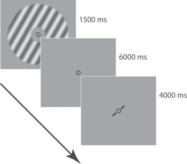
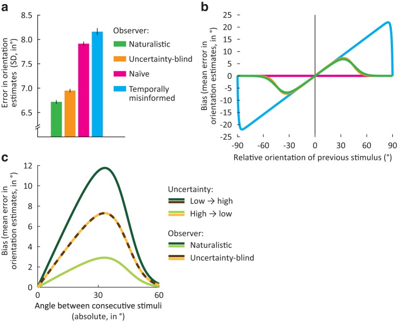
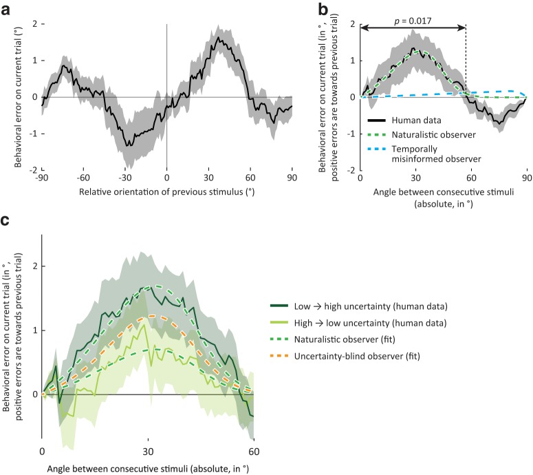
How does the brain represent the reliability of its sensory evidence? Here, we test whether sensory uncertainty is encoded in cortical population activity as the width of a probability distribution, a hypothesis that lies at the heart of Bayesian models of neural coding. We probe the neural representation of uncertainty by capitalizing on a well-known behavioral bias called serial dependence. Human observers of either sex reported the orientation of stimuli presented in sequence, while activity in visual cortex was measured with fMRI. We decoded probability distributions from population-level activity and found that serial dependence effects in behavior are consistent with a statistically advantageous sensory integration strategy, in which uncertain sensory information is given less weight. More fundamentally, our results suggest that probability distributions decoded from human visual cortex reflect the sensory uncertainty that observers rely on in their decisions, providing critical evidence for Bayesian theories of perception.SIGNIFICANCE STATEMENT Virtually any decision that people make is based on uncertain and incomplete information. Although uncertainty plays a major role in decision-making, we have but a nascent understanding of its neural basis. Here, we probe the neural code of uncertainty by capitalizing on a well-known perceptual illusion. We developed a computational model to explain the illusion, and tested it in behavioral and neuroimaging experiments. This revealed that the illusion is not a mistake of perception, but rather reflects a rational decision under uncertainty. No less important, we discovered that the uncertainty that people use in this decision is represented in brain activity as the width of a probability distribution, providing critical evidence for current Bayesian theories of decision-making.

Keywords: computational modeling; fMRI; perceptual decision-making; serial dependence; uncertainty.

Figure 1.

Trial structure. Each trial in the experiment started with the presentation of a stimulus, followed by a fixation interval, and then a response window. Trials were separated by a 4000 ms intertrial interval. Participants adjusted the orientation of a centrally presented bar to match the previously seen stimulus orientation. The stimulus and response bar are not drawn to true scale and contrast.

Figure 2.

Distribution of orientation change over time in natural videos. Two databases of natural videos, which we refer to as cat and city (Kayser et al., 2003; Betsch et al., 2004; Dorr et al., 2010), were analyzed for their orientation content as it evolved over time. Each video database was analyzed at three different spatial scales (lower, middle, and upper third of the spatial frequency spectrum) and for three different temporal intervals (200, 1000, and 10,000 ms). Panels represent the orientation transition distribution measured in the two databases for different temporal intervals (averaged across spatial scales) and spatial scales (averaged across temporal intervals), as well as the overall mean across all spatial and temporal scales and both databases. The general shape observed across all analysis settings is that of a flat baseline with a central peak, which in the naturalistic observer model was approximated by a mixture distribution of a central peak and a uniform baseline.

Figure 3.

Effect of parameter values on modeled serial dependence bias. Model behavior was simulated using various parameter values to illustrate the range of serial dependence curves predicted by each of the observer models. Panels represent the magnitude of the error on the current trial as a function of the absolute difference in orientation between current and previous stimuli. Positive bias values reflect errors toward the previously presented stimulus, and data are the mean error across trials. Biases are shown for the naturalistic and temporally misinformed observers. By definition, the serial dependence bias of the naive observer is zero, regardless of orientation angle, and is not shown here. When averaged across uncertainty levels, the bias curve of the naturalistic observer is virtually identical to that of the uncertainty-blind observer (see Fig. 5b), which is why the latter is not shown here. Trial-by-trial fluctuations in uncertainty change the magnitude, but not the shape, of the bias curve (see Fig. 5c). Parameter values were manipulated around default settings of μ_avg = 8°, p_same = 0.5, σ_s = 10°, and γ = 2. In each plot, the medium gray curve corresponds to these default parameters and is identical between panels (for the same observer). Parameters p_same and γ are not free parameters in the temporally misinformed observer model and were not manipulated there. For the temporally misinformed observer, the serial dependence bias only equals 0 when orientations differ by exactly 90°; whereas for the naturalistic model observer, the no-bias point can be reached much earlier, depending on parameter values. This is because the temporally misinformed observer invariably averages together previous and current sensory observations, regardless of their orientation difference. Consequently, the serial bias of this observer is only 0 when the circular average of these orientations is 0 (i.e., when orientations are orthogonal). The different values of γ correspond to excess kurtoses of 3 (Laplacian), 0 (Gaussian), and −0.8 (sub-Gaussian), for γ = 1, 2, and 4, respectively. For the default setting of γ = 2, σ_s corresponds to the standard deviation (SD) of the central peak in the transition model. When γ is set to different values, however, this changes both the kurtosis and SD of the central peak. To illustrate the specific effect of changing kurtosis, σ_s was therefore adjusted along with γ to keep the SD fixed at an approximately constant value of 10°. As evident from the resulting plots, changing the kurtosis of the central peak does not strongly affect the shape of the serial dependence curve. This is because the transition distribution is convolved with an (approximately) Gaussian distribution (reflecting the observer's knowledge about the previous stimulus), which smoothens the central peak. The result of this convolution is the observer's prediction, which, for a reasonable range of kurtosis values of the transition distribution, always tends toward a Gaussian shape.

Figure 4.

Ideal observer in the natural environment. Illustration represents a single iteration in a continuous perceptual inference cycle. Left column represents the degree to which the environment remains stable over time, described by the transition model (light blue). For instance, edges in the environment (e.g., the one marked in orange) typically do not change much from one moment to the next. The ideal observer uses knowledge of these transition probabilities to infer the stimulus from its noisy sensory inputs. Specifically, at time t = 0, the observer takes a sensory measurement m⁽⁰⁾ of the stimulus s⁽⁰⁾ (an oriented edge). The measurement carries information about the stimulus, which is expressed by the probability distribution p(s⁽⁰⁾|m⁽⁰⁾) (yellow). This distribution is subsequently combined with a prediction (pink), which is based on previous sensory observations combined with knowledge of the environment's temporal statistics. The prediction is expressed by a probability distribution p(s⁽⁰⁾|m^(t₀:−1)), where t₀ denotes the starting point of the inference process that is arbitrarily long ago. The prediction is integrated with incoming sensory information to arrive at a combined distribution p(s⁽⁰⁾|m^(t₀:0)) (red), which reflects all sources of knowledge available to the observer at t = 0. Finally, the observer uses this perceptual knowledge available at time 0 to generate a new prediction p(s⁽¹⁾|m^(t₀:0)) (purple) about the next stimulus at time t = 1, and the cycle continues.

Figure 5.

Simulated behavior of various observer models in an orientation estimation task. a, Error standard deviation (SD) in orientation estimates for each of four model observers on sequences of orientation stimuli that were generated using naturalistic temporal statistics (i.e., correlations over time). The ideal or naturalistic observer uses knowledge of temporal stimulus statistics while taking into account the uncertainty associated with successive stimulus estimates. The uncertainty-blind observer similarly combines previous and current sensory estimates but fails to weight each by its associated uncertainty. The naive observer bases estimates solely on sensory input from the current trial. The temporally misinformed observer takes into account uncertainty but assumes an incorrect model of temporal statistics. The naturalistic observer outperforms the other three model observers that each ignore important aspects of the optimal inference process. Error bars indicate bootstrapped 95% confidence intervals. b, When presented with stimuli that are uncorrelated over time, the naturalistic observer incorrectly assumes temporal dependencies, and as a result, gives estimates that are biased toward previously seen stimuli (green). The same is true for the uncertainty-blind observer (orange), whose biases are nearly identical to those of the naturalistic observer (when averaged across uncertainty levels, as in this plot). This is in contrast to an observer model that assumes uncorrelated stimuli (the naive observer); the estimates of this observer model exhibit no biases at all (pink). The temporally misinformed observer, on the other hand, does produce biased estimates but combines current and previous estimates regardless of their difference in orientation (blue). For a detailed analysis of model parameters and their effects on predicted behavior, see Materials and Methods. Plotted is the predicted bias in the orientation estimates of the model observer as a function of the orientation of the previous relative to the current stimulus (acute-angle difference between previous and current orientation). For both axes, positive angles are in a clockwise direction. c, For the uncertainty-aware naturalistic model observer, the bias is stronger when the observer is less uncertain about the previously seen stimulus than the current stimulus (dark green), than when the current sensory information was most reliable in comparison (light green). For the uncertainty-blind observer, the bias is identical across levels of uncertainty (brown and yellow). Plotted is the predicted bias as a function of the absolute orientation difference between current and previous trial. Positive bias values reflect errors toward the previous trial's orientation.

Figure 6.

Human behavior matches the predictions of the naturalistic observer model. a, Group-average behavioral errors, smoothed with a moving average filter, as a function of the relative orientation presented on the previous trial. Positive errors and orientation differences are in the clockwise direction. In this and subsequent panels, solid line and shaded region represent the mean ± SEM across observers. b, Same as in a, but with behavioral errors realigned such that positive deviations are in the direction of the orientation presented on the previous trial, and plotted against the absolute, rather than the signed, difference in orientations. Arrows indicate the extent of orientation differences for which a cluster-based analysis revealed a significant bias in the direction of the previous trial (p = 0.017). A small negative serial dependence bias is also apparent for orientation angles > ±60° but did not reach statistical significance (p = 0.079, cluster-based permutation test). Green curve indicates the optimal fit of the naturalistic ideal observer model to the behavioral data. This model explains significant variance in the data (R² = 0.86, p = 0.02). Blue curve indicates the optimal fit of an alternative observer model ignoring natural temporal statistics. The bias curve generated by this model is very different in shape from that observed in human behavior, and does not capture the human data well (R² = 0.02, p = 0.41). c, Similar to the naturalistic observer, the serial dependence bias in human behavior is stronger when the sensory representation is more uncertain on the current than previous trial (dark green), compared with when sensory information is less uncertain now than in the recent past (light green; t₍₁₇₎ = 2.96, p = 0.009). Dashed curves indicate the optimal fit of the naturalistic observer (green) and uncertainty-blind observer models (orange). The naturalistic observer model explained significantly more variance than a model ignoring fluctuations in uncertainty (R² increase from 0.65 to 0.78, p = 0.01), suggesting that, like the naturalistic observer model, human observers integrate current and previous sensory inputs in an uncertainty-weighted manner.

References

1. Alais D, Burr DC (2004) The ventriloquist effect results from near-optimal bimodal integration. Curr Biol 14:257–262. 10.1016/j.cub.2004.01.029 - DOI - PubMed
1. Anastasio TJ, Patton PE, Belkacem-Boussaid K (2000) Using Bayes' rule to model multisensory enhancement in the superior colliculus. Neural Comput 12:1165–1187. 10.1162/089976600300015547 - DOI - PubMed
1. Appelle S. (1972) Perception and discrimination as a function of stimulus orientation: the “oblique effect” in man and animals. Psychol Bull 78:266–278. 10.1037/h0033117 - DOI - PubMed
1. Battaglia PW, Jacobs RA, Aslin RN (2003) Bayesian integration of visual and auditory signals for spatial localization. J Opt Soc Am A 20:1391. 10.1364/JOSAA.20.001391 - DOI - PubMed
1. Betsch BY, Einhäuser W, Körding KP, König P (2004) The world from a cat's perspective: statistics of natural videos. Biol Cybern 90:41–50. 10.1007/s00422-003-0434-6 - DOI - PubMed
Publication types
LinkOut - more resources