High-Throughput Single-Cell Sequencing with Linear Amplification

Abstract

Conventional methods for single-cell genome sequencing are limited with respect to uniformity and throughput. Here, we describe sci-L3, a single-cell sequencing method that combines combinatorial indexing (sci-) and linear (L) amplification. The sci-L3 method adopts a 3-level (3) indexing scheme that minimizes amplification biases while enabling exponential gains in throughput. We demonstrate the generalizability of sci-L3 with proof-of-concept demonstrations of single-cell whole-genome sequencing (sci-L3-WGS), targeted sequencing (sci-L3-target-seq), and a co-assay of the genome and transcriptome (sci-L3-RNA/DNA). We apply sci-L3-WGS to profile the genomes of >10,000 sperm and sperm precursors from F1 hybrid mice, mapping 86,786 crossovers and characterizing rare chromosome mis-segregation events in meiosis, including instances of whole-genome equational chromosome segregation. We anticipate that sci-L3 assays can be applied to fully characterize recombination landscapes, to couple CRISPR perturbations and measurements of genome stability, and to other goals requiring high-throughput, high-coverage single-cell sequencing.

Keywords: DNA repair; chromosome segregation; double-strand break; homologous recombination; infertility; linear amplification; meiotic crossover; mouse; single-cell combinatorial indexing; single-cell sequencing.

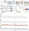
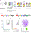
Figure 1.. sci-L3-WGS enables high-throughput single cell sequencing with linear amplification.

(A) sci-L3-WGS workflow. (B) Top: barcode structure of resulting DNA duplexes. bc, barcode; sp, spacer; gDNA, genomic DNA. Middle: example library structure for sci-L3-WGS. P5 and P7 sequencing adaptors are added by A-tailing and ligation. Note that having P7 on the UMI end and P5 on the gDNA end are equally possible due to symmetry of ligation. Bottom: example library structure for sci-L3-target-seq. P5 and P7 sequencing adaptors are added by priming from spacer 2 (sp2) and targeted loci of interest in the genome, respectively. Note that a new third round of barcode bc3’ is also added by PCR corresponding to each bc3 in the WGS library, and new UMI’ are added outside of bc3’. (C) Scatter plot of numbers of unique Tn5 insertions from human and mouse cells at low sequencing depth, 24 bc1 × 64 bc2 × 6 bc3 sci-L3-WGS, 100 to 300 cells sorted per well. Blue, inferred mouse cells (% of mouse reads >95%; median 98.7%; n=315); red, inferred human cells (% of human reads >95%; median 99.8%; n=719); grey, inferred collisions (n=48; 4% of cells). ‘Contaminating’ reads arise randomly throughout the genome (Figure S1H). (D) Box plots showing number of unique Tn5 insertions per cell at mean 2.4M raw reads per cell and 1.78x depth. Depth defined as ratio of unique IVT transcripts to unique Tn5 insertions. Thick horizontal lines, medians; upper and lower box edges, first and third quartiles, respectively; whiskers, 1.5 times the interquartile range; circles, outliers). See Figure S1 and STAR Methods, “Methods and molecular design of sci-L3-WGS and sci-L3-target-seq” for characterization of libraries made with improved versions of protocol. (E) Example chromosome CNV plots for individual cells. Upper, HEK293T cell, 2.6M raw reads, 2.4M unique molecules, 1.3M unique Tn5 insertions with MAPQ > 1. Lower, 3T3 cell, 2.7M raw reads, 2.4M unique molecules, 1.2M unique Tn5 insertions with MAPQ > 1. (F) Box plots for copy number variation across 822 293T cells or 1,453 HAP1 cells. Y-axis depicts reads fraction per chromosome normalized by chromosome length such that a euploid chromosome without segmental copy gain or loss is expected to have a value of 1.

Figure 2.. Molecular structures for sci-LIANTI at each step.

Dashed line: RNA, solid line: DNA. (A) Tn5 adaptors have both 5’ ends phosphorylated, one required for insertion and the other for ligation. The overhang of the annealed transposon contains first round barcodes (bc1) and a spacer (sp1) for ligation. (B) The ligation molecule is pre-annealed as a hairpin loop, which reduces intermolecular ligation from three molecules to two molecules; the hairpin structure also helps improve RT efficiency in downstream steps. The hairpin contains: 1) an overhang that anneals with sp1 for ligation, 2) the second round barcodes (bc2) and a spacer (sp2) that serves as a priming site in the stem for SSS in downstream steps, and 3) a T7 promoter in the loop for IVT. (C) Gap extension converts the looped T7 promoter to a duplex. Note that if ligation is successful on both ends, T7 promoters are present on both sides; however, if ligation is successful on one end, the boxed portion will be missing. Nevertheless, both can be reverse transcribed in downstream steps with different RT primers. (D) IVT generates single-stranded RNA amplicons downstream of the T7 promoter. (E) If ligation was successful on both ends, RT is preferably primed by self-looped RT primers, which are inherited from the looped ligation molecule; if ligation was successful on only one end, RT is primed by additional RNA RT primers added in excess. Excess RNA primers are then removed before SSS to avoid interfering with SSS reaction. (F) Double-stranded DNA molecules are produced by SSS which primes off sp2 to simultaneously add the third barcode and to UMI tag each transcript. For more details, see STAR Methods, “Methods and molecular design of sci-L3-WGS and sci-L3-target-seq”.

Figure 3.. Sci-L3-based RNA/DNA co-assay enables scalable, joint profiling of single cell genomes and transcriptomes.

(A) Schematic of sci-L3-RNA/DNA co-assay. Note that both Tn5 transposon and cDNA synthesis primer contain the same phosphorylated ligation landing pad (pink) at 5’ overhang outside of first round barcodes. (B) Barcode structures of resulting amplified duplexes corresponding to genome (left) and transcriptome (right). (C) Scatter plot of numbers of unique Tn5 insertions from human and mouse cells at low and high sequencing depth plotted together. Blue, inferred mouse cells (% mouse reads >95%, median of 99.5%; n=2002); red, inferred human cells (% human reads >95%; median of 99.8%; n=2419); grey, inferred collisions (n=149; 6.6%). (D) Same as in (C) for RNA. Blue, inferred mouse cells (median purity 95.1%); red, inferred human cells (median purity 91.5%); grey, inferred collisions (n=272; 12%). (E) t-SNE based on RNA profiles results in two clusters corresponding to BJ (male) and HEK293T (female) cells. Colors based on presence or absence of Y chromosomes in DNA profiles.

Figure 4.. sci-L3-WGS of interspecific hybrid mouse male germline reveals numerous examples of non-independent equational segregation in MI.

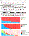
In (A), (B) and (C), red line depicts fitted crossover transition via HMM. Centromere is located at the leftmost for picture of each chromosome. (A) Example crossover plot for 1C cell. Grey dot has a value of 1 for Spret allele and 0 for B6 allele. In (B) and (C), grey dot shows allele frequency of Spret averaging 40 SNPs. (B) Example LOH plot for M2 cell with reductional segregation (see also Figure S2D): LOH centromere-proximal to the crossover. (C) Example LOH plot for M2 cell with equational segregation (see also Figure S2B): LOH centromere-distal to the crossover, unlike in (B). (D-F) Number of reductionally (red, pink, black) and equationally (blue, green) segregated chromosomes for each M2 cell. Each column represents one M2 cell (19 chromosomes per cell, distributed as indicated by colors). (D) Expected distribution of reductional vs. equational segregation based on binomial distribution with p=0.76 for reductional segregation. (E) Observed data in M2 cells. In rare cases (27/5,548 chromosomes), we were not able to distinguish reductional vs. equational segregation due to sparse SNP coverage (white space at the top of the panel). Black bar depicts MI nondisjunction (NDJ, 40 chromosomes in total) where we observed 0 or 4 copies of the chromatids. Note that NDJ is considered as reductional segregation because the sister chromatids segregate together. (F) Same as (E) but further broken down by the number of chromosomes with or without crossovers (abbreviated as “CO”). Cells are sorted first by number of equationally segregated chromosomes (light green and blue, in descending order) and then by number of observed equationally segregated chromosomes without crossover (blue, in descending order).

Figure 5.. sci-L3-WGS of the intraspecific hybrid mouse male germline also reveals numerous examples of non-independent equational segregation.

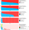
(A-B) Number of reductionally and equationally segregated chromosomes for artificial “2C” cells from barcode group 1, which derive from doublets of two random 1C cells. Same depiction as in Figure 4. (A) Expected distribution of reductional vs. equational segregation based on the binomial distribution and assuming the probability of equational segregation p equals 0.5. (B) Observed data in 2C cells, which matches the expected distribution shown in (A). (C-E) Number of reductionally and equationally segregated chromosomes for non-1C cells from barcode group 2, which are a mixture of both artificial doublets of two random 1C nuclei and real 2C secondary spermatocytes. (C) All non-1C cells from barcode group 2. (D) Non-1C cells with biased chromosome segregation only, i.e., ≥15 chromosomes segregated either equationally or reductionally. Black bar depicts Meiosis I NDJ (2 of 2,185 chromosomes). (E) Same as (D) but further broken down by the number of chromosomes with or without crossovers.

Figure 6.. Meiotic crossover hotness and explanatory genomic features.

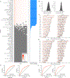
(A) Marginal inclusion probability (MIP) for features associated with crossover hotness by BMA. The x-axis ranks models by posterior probability, where grey boxes depict features not included in each model (vertical line, 20 top models are shown) and orange color scale depicts posterior probability of the models. The combined dataset from both the (B6 × Spret) and (B6 × Cast) crosses is shown here. See Figure S5 for the two crosses analyzed separately. (B) Log normal distribution of sizes for breakpoint resolution. Left: (B6 × Spret), median of 150 kb. Right: (B6 × Cast), median of 250 kb. (C-D) Positions of the rightmost crossover of each chromosome. (C) M2 cell. Crossovers in the (B6 × Cast) (left) cross prefer the centromere-distal end of the chromosome, while crossovers in the (B6 × Spret) cross (right) prefer the middle region of each chromosome arm. After accounting for inter-chromosome variability, we estimate that crossovers in the (B6 × Spret) cross are on average 5.5 Mb more centromere-proximal. See Figure S7A which is similar but for 1C cells. (D) Comparing 1C and M2 cells, (B6 × Spret) cross. After accounting for inter-chromosome variability, we estimate that crossovers in M2 cells (right) are on average 9.4 Mb more centromere-proximal than in 1Cs (left) in the (B6 × Spret) cross. The same trend is observed to a lesser extent in the (B6 × Cast) cross (see Figure S7B). (E) AUC of 0.73 quantifies expected accuracy in predicting if a region drawn from the mouse genome comes from B6 × Spret crossover tracts or an equal number of randomly sampled tracts. Left: all 76 features. Right: a subset of 25 features from BMA with MIP>0.5. (F) AUC of 0.85 quantifies expected accuracy in predicting if a region drawn from the mouse genome comes from B6 × Cast crossover tracts or an equal numbers of randomly sampled tracts. Left: all 69 features. Right: a subset of 25 features from BMA with MIP>0.5.

References

1. Barrai S, Morozumi Y, Tanaka H, Montellier E, Govin J, de Dieuleveult M, Charbonnier G, Couté Y, Puthier D, Buchou T, et al. (2017). Histone Variant H2A.L.2 Guides Transition Protein-Dependent Protamine Assembly in Male Germ Cells. Mol. Cell 66, 89–101.e8. - PubMed
1. Baudat F, Manova K, Yuen JP, Jasin M, and Keeney S (2000). Chromosome synapsis defects and sexually dimorphic meiotic progression in mice lacking Spoil. Mol. Cell 6, 989–998. - PubMed
1. Baudat F, Imai Y, and de Massy B (2013). Meiotic recombination in mammals: localization and regulation. Nat. Rev. Genet 14, 794–806. - PubMed
1. Berletch JB, Ma W, Yang F, Shendure J, Noble WS, Disteche CM, and Deng X (2015). Escape from X inactivation varies in mouse tissues. PLoS Genet. 11, e1005079. - PMC - PubMed
1. de Boer E, Jasin M, and Keeney S (2015). Local and sex-specific biases in crossover vs. noncrossover outcomes at meiotic recombination hot spots in mice. Genes Dev. 29, 1721–1733. - PMC - PubMed
Publication types
LinkOut - more resources