Consistent and correctable bias in metagenomic sequencing experiments

Abstract

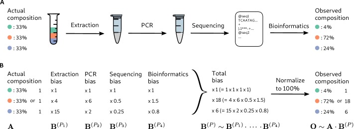
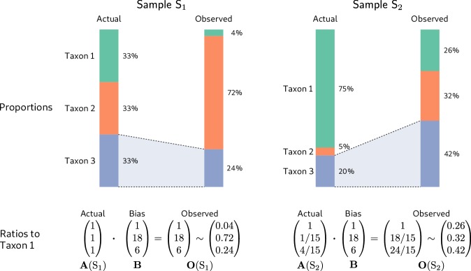
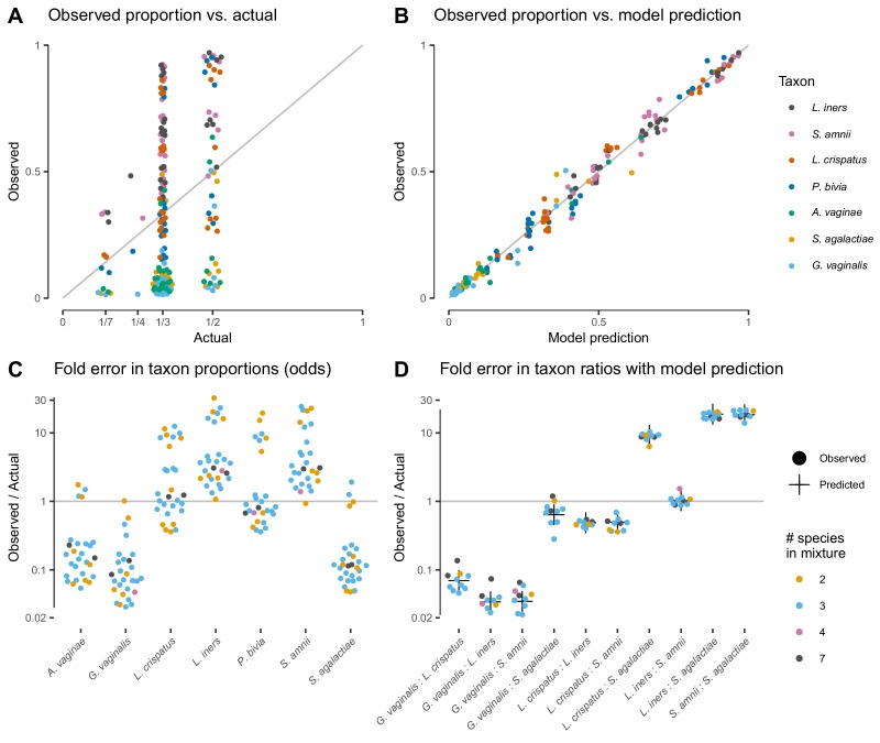
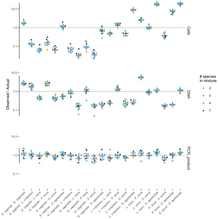
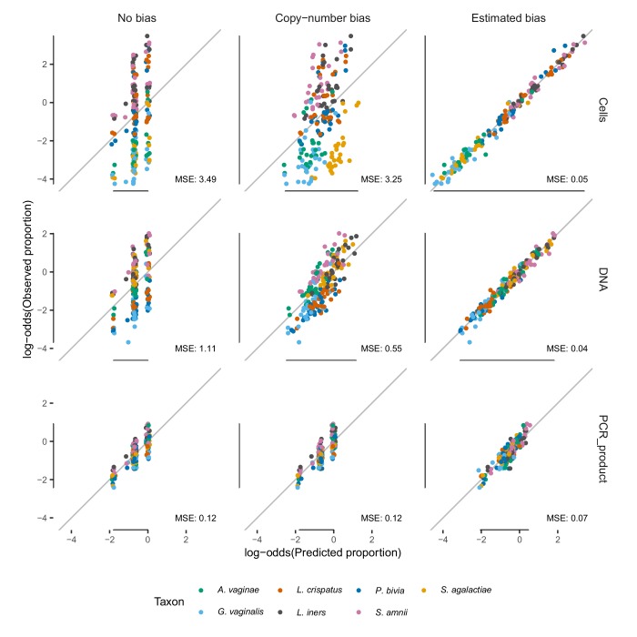
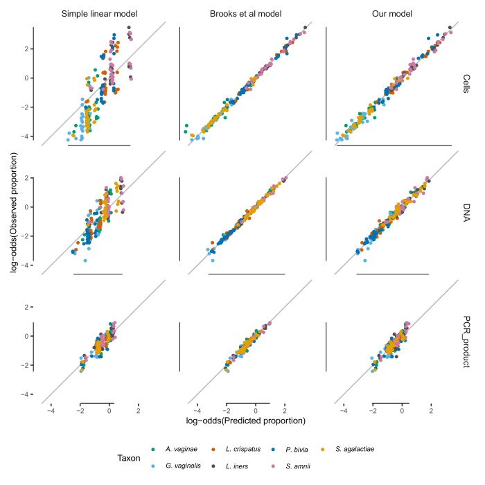
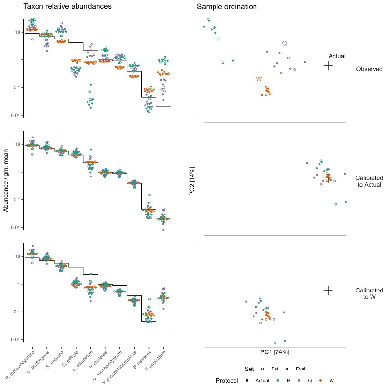
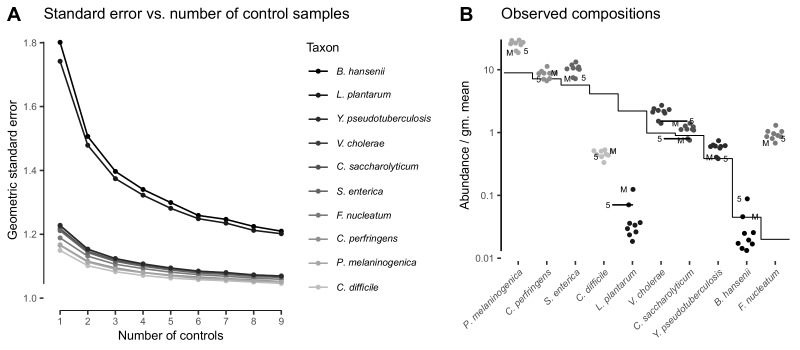
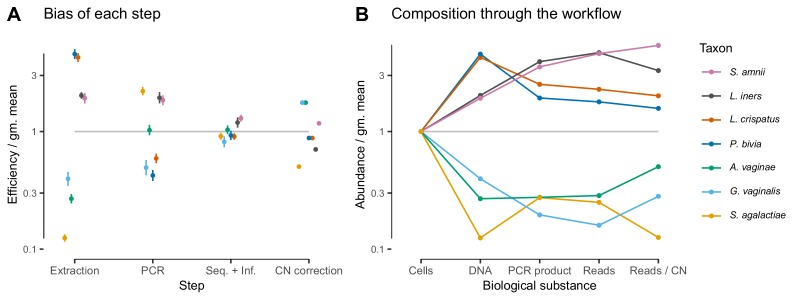
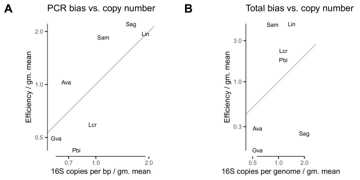
Marker-gene and metagenomic sequencing have profoundly expanded our ability to measure biological communities. But the measurements they provide differ from the truth, often dramatically, because these experiments are biased toward detecting some taxa over others. This experimental bias makes the taxon or gene abundances measured by different protocols quantitatively incomparable and can lead to spurious biological conclusions. We propose a mathematical model for how bias distorts community measurements based on the properties of real experiments. We validate this model with 16S rRNA gene and shotgun metagenomics data from defined bacterial communities. Our model better fits the experimental data despite being simpler than previous models. We illustrate how our model can be used to evaluate protocols, to understand the effect of bias on downstream statistical analyses, and to measure and correct bias given suitable calibration controls. These results illuminate new avenues toward truly quantitative and reproducible metagenomics measurements.

Keywords: 16S rRNA gene; bias; calibration; computational biology; infectious disease; metagenomics; microbiology; microbiome; reproducibility; systems biology.

Figure 1.. Bias arises throughout an MGS workflow, creating systematic error between the observed and actual compositions.

Panel A illustrates a hypothetical marker-gene measurement of an even mixture of three taxa. The observed composition differs from the actual composition due to the bias at each step in the workflow. Panel B illustrates our mathematical model of bias, in which bias multiplies across steps to create the bias for the MGS protocol as a whole.

Figure 2.. Consistent multiplicative bias causes systematic error in taxon ratios, but not taxon proportions, that is independent of sample composition.

The even community from Figure 1 and a second community containing the same three taxa in different proportions are measured by a common MGS protocol. Measurements of both samples are subject to the same bias, but the magnitude and direction of error in the taxon proportions depends on the underlying composition (top row). In contrast, when the relative abundances and bias are both viewed as ratios to a fixed taxon (here, Taxon 1), the consistent action of bias across samples is apparent (bottom row).

Figure 3.. Our model of bias explains the systematic error observed in the Brooks et al. (2015) cell-mixture experiment.

The top row compares the observed proportions of individual taxa to the actual proportions (Panel A) and to those predicted by our fitted bias model (Panel B). Panel A shows significant error across all taxa and mixture types that is almost entirely removed once bias is accounted for in Panel B. Panel C shows the observed error in proportions of individual taxa, while Panel D shows the error in the ratios of pairs of taxa for five of the seven taxa. The ratio predicted by the fitted model is given by the black cross in Panel D. As predicted by our model, the error in individual proportions (Panel C) depends highly on sample composition, while the error in ratios (Panel D) does not.

Figure 3—figure supplement 1.. The observed error in taxon ratios for all three mixture experiments.

The observed error in taxon ratios (colored dots) against the fitted model prediction (black cross) for the three mixture experiments of Brooks et al. (2015).

Figure 3—figure supplement 2.. Observed vs. expected proportions under no bias, copy-number bias only, and the estimated bias.

Comparison of the observed proportions with three types of expected proportions—the actual proportions, the proportions predicted from the estimated 16S copy numbers in Table 3, and the proportions predicted by the fitted bias model—for the three mixture experiments of Brooks et al. (2015). Proportions $p$ are transformed to log-odds ($\ln [p/(1-p)]$) to avoid compressing errors near $p=0$ and $p=1$, and average mean squared error (MSE) of the log-odds are shown.

Figure 3—figure supplement 3.. Comparison between the simple linear model, the linear interactions model of Brooks et al. (2015), and our model.

Comparison of the model fits for the simple linear model, the linear interactions model of Brooks et al. (2015), and our model. The simple linear model has a poor fit, while the Brooks et al. (2015) model closely fits the data but does so by having more parameters per taxon (63 per taxon) than distinct sample compositions (58). Our model fits nearly as well as the Brooks et al. (2015) model for the Cells and DNA mixtures, while having vastly fewer parameters (6 versus 441 for all taxa). Proportions $p$ are transformed to log-odds ($\ln [p/(1-p)]$) to avoid compressing errors near $p=0$ and $p=1$. The simple linear model with and without an intercept term gives nearly identical results except near zero; here shown without. Only taxa with non-zero actual abundance are plotted, and proportions predicted to be greater than one by the simple linear model are not shown.

Figure 4.. Bias of the mock spike-in in the Costea et al. (2017) experiment is consistent across samples with varying background compositions.

Panel A shows the variation in bacterial composition across protocols and specimens (Labels 1 through 8 denote fecal specimens; M denotes the mock-only specimen) and Panel B shows the relative abundance of the 10 mock taxa and the spike-in contaminant (dots) against the actual composition (black line). In Panel A, color indicates source (mock, contaminant, or native gut taxon) and Family for native bacterial taxa with a proportion of 0.02 in at least one sample. Families are colored by phylum (Red: Actinobacteria, Green: Bacteroidetes, Blue: Firmicutes, Orange: Verrucomicrobia). In Panel B, abundance is divided by the geometric mean of the mock (non-contaminant) taxa in that sample.

Figure 4—figure supplement 1.. Estimated bias for the mock taxa for the three protocols.

Estimated bias for the 10 mock taxa for the three protocols in the Costea et al. (2017) experiment. Bias is shown as relative to the average taxon; that is, the efficiency of each taxon is divided by the geometric mean efficiency of all taxa. The estimated efficiencies are shown as the best estimate (dark dot) multiplied and divided by two geometric standard errors (lines), along with the observations from individual samples (translucent dots).

Figure 5.. Calibration can remove bias and make MGS measurements from different protocols quantitatively comparable.

For the sub-community defined by the mock spike-in of the Costea et al. (2017) dataset, we estimated bias from three specimens (the estimation set ‘Est’) and used the estimate to calibrate all specimens. The left column shows taxon relative abundances as in Figure 4B and the right column shows the first two principal components from a compositional principle-components analysis (Gloor et al., 2017). The top row shows the measurements before calibration; the middle, after calibration to the actual composition; and the bottom, after calibration to Protocol W.

Figure 5—figure supplement 1.. Precision in the bias estimate vs. the number of control samples for Protocol H.

Precision in bias estimate decreases with the number of control samples and depends on the noise associated with each taxon. For Protocol H in the Costea et al. (2017) experiment, Panel A shows the geometric standard error in the relative efficiencies of the 10 mock taxa (which jointly form the estimated bias) versus the number of control samples used to estimate the bias. As elsewhere, the efficiency of each taxon is divided by the geometric mean efficiency of all 10 mock taxa. Panel B shows the observed against the actual relative abundances, as in Figure 4. The two marked samples (from Individual 5 and the mock-only sample M) have unusually high observed abundances of L. plantarum and B. hansenii and are largely responsible for the much higher standard error seen for these two taxa.

Figure 6.. In the Brooks et al. (2015) experiment, bias is primarily driven by DNA extraction and is not substantially reduced by 16S copy-number (CN) correction.

Panel A shows the bias estimate for each step in the experimental workflow (DNA extraction, PCR amplification, and sequencing + (bio)informatics), as well as the bias imposed by performing 16S CN correction (i.e. dividing by the estimated number of 16S copies per genome). Bias is shown as relative to the average taxon—that is, the efficiency of each taxon is divided by the geometric mean efficiency of all seven taxa—and the estimated efficiencies are shown as the best estimate multiplied and divided by two geometric standard errors. Panel B shows the composition through the workflow, starting from an even mixture of all seven taxa, obtained by sequentially multiplying the best estimates in Panel A.

Figure 6—figure supplement 1.. PCR bias and total bias vs. bias predicted by 16S copy number.

In the Brooks et al. (2015) experiment, variation in 16S copy number is moderately predictive of PCR bias (A) but not of total bias (B). The grey line corresponds to $y=x$, or perfect agreement between CN and the estimated bias.

Author response image 1.

References

1. Aitchison J. The Statistical Analysis of Compositional Data. London: Chapman and Hall; 1986.
1. Aitchison J. On criteria for measures of compositional difference. Mathematical Geology. 1992;24:365–379. doi: 10.1007/BF00891269. - DOI
1. Aitchison J. A concise guide to compositional data analysis. 2nd Compositional Data Analysis Workshop; 2003.
1. Barceló-Vidal C, Martín-Fernández JA, Pawlowsky-Glahn V. Mathematical foundations of compositional data analysis. Proceedings of IAMG'01—The Sixth Annual Conference of the International Association for Mathematical Geology; 2001.
1. Bell KL, Burgess KS, Botsch JC, Dobbs EK, Read TD, Brosi BJ. Quantitative and qualitative assessment of pollen DNA metabarcoding using constructed species mixtures. Molecular Ecology. 2019;28:431–455. doi: 10.1111/mec.14840. - DOI - PubMed