Automated, unsupervised inversion of multiwavelength lidar data with TiARA: assessment of retrieval performance of microphysical parameters using simulated data

Abstract

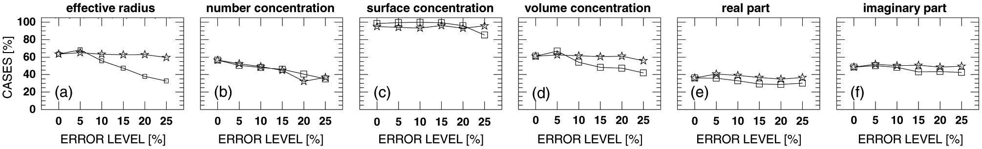
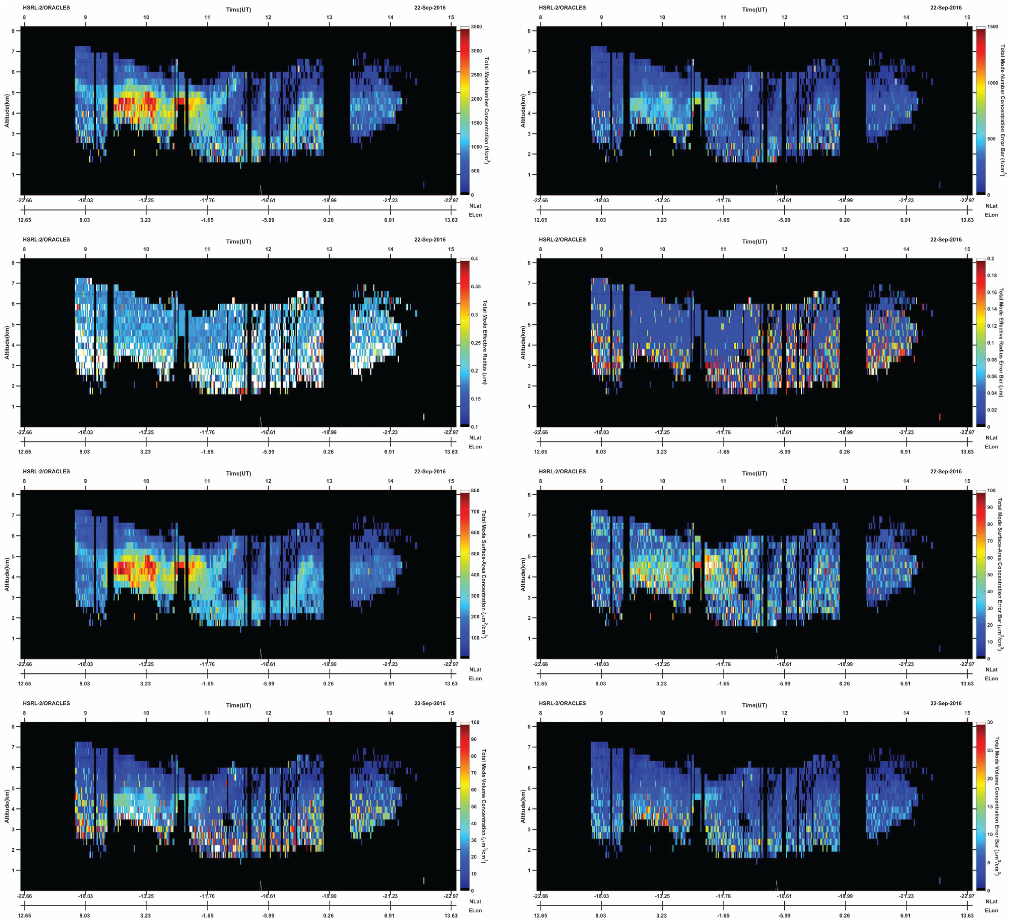
We evaluate the retrieval performance of the automated, unsupervised inversion algorithm, Tikhonov Advanced Regularization Algorithm (TiARA), which is used for the autonomous retrieval of microphysical parameters of anthropogenic and natural pollution particles. TiARA (version 1.0) has been developed in the past 10 years and builds on the legacy of a data-operator-controlled inversion algorithm used since 1998 for the analysis of data from multiwavelength Raman lidar. The development of TiARA has been driven by the need to analyze in (near) real time large volumes of data collected with NASA Langley Research Center's high-spectral-resolution lidar (HSRL-2). HSRL-2 was envisioned as part of the NASA Aerosols-Clouds-Ecosystems mission in response to the National Academy of Sciences (NAS) Decadal Study mission recommendations 2007. TiARA could thus also serve as an inversion algorithm in the context of a future space-borne lidar. We summarize key properties of TiARA on the basis of simulations with monomodal logarithmic-normal particle size distributions that cover particle radii from approximately 0.05 μm to 10 μm. The real and imaginary parts of the complex refractive index cover the range from non-absorbing to highly light-absorbing pollutants. Our simulations include up to 25% measurement uncertainty. The goal of our study is to provide guidance with respect to technical features of future space-borne lidars, if such lidars will be used for retrievals of microphysical data products, absorption coefficients, and single-scattering albedo. We investigate the impact of two different measurement-error models on the quality of the data products. We also obtain for the first time, to the best of our knowledge, a statistical view on systematic and statistical uncertainties, if a large volume of data is processed. Effective radius is retrieved to 50% accuracy for 58% of cases with an imaginary part up to 0.01i and up to 100% of cases with an imaginary part of 0.05i. Similarly, volume concentration, surface-area concentration, and number concentrations are retrieved to 50% accuracy in 56%-100% of cases, 99%-100% of cases, and 54%-87% of cases, respectively, depending on the imaginary part. The numbers represent measurement uncertainties of up to 15%. If we target 20% retrieval accuracy, the numbers of cases that fall within that threshold are 36%-76% for effective radius, 36%-73% for volume concentration, 98%-100% for surface-area concentration, and 37%-61% for number concentration. That range of numbers again represents a spread in results for different values of the imaginary part. At present, we obtain an accuracy of (on average) 0.1 for the real part. A case study from the ORCALES field campaign is used to illustrate data products obtained with TiARA.

Fig. 1.

(left) Example of the qualitative reconstruction of a PSD with five base functions of triangular shape distributed in the radius interval [r_min, r_max]. The radius interval is denoted as inversion window in the text. (right) We use eight base functions in our algorithm, as it allows us also to reconstruct bimodal size distributions.

Fig. 2.

(top) Gliding inversion window. We show the arrangement of the nine inversion windows. (bottom) Grid of the complex refractive indices.

Fig. 3.

Example of the linear combination of three optimized LUT base functions $b_{j_1}(r)$, $b_{j_1+1}(r)$, and $b_{j_1+2}(r)$ into one inversion triangular base function B_j(r).

Fig. 4.

Illustration of (top) extreme-error model (EEM) and (bottom) Gauss-error model (GEM).

Fig. 5.

Flowchart of TiARA. The meanings of the numbers in circles in the flowchart are given in Appendix A.

Fig. 6.

PSDs that were tested in our simulation studies.

Fig. 7.

Graphical display of effective radius and surface-area and volume concentrations of the PSDs that were used for the computation of the optical data used in the simulations. Each symbol represents one specific combination of median radius and geometrical standard deviation. The numerical vales of the parameters are given in Appendix A.

Fig. 8.

Example of retrieval performance for the case of size distributions with a geometrical standard deviation of 1.9 and median radii of 20 nm, 60 nm, 100 nm, 140 nm, 180 nm, 220 nm, 206 nm, and 300 nm (Table 5). We tested all 15 imaginary parts of the complex refractive index of the investigated particle size distributions (Table 5).We show the results for the imaginary parts 0i, 0.005i, 0.01i, 0.03i, and 0.05i. Each data point (with error bar) shows the average and standard deviation of multiple solutions in one retrieval. The first row shows the results for effective radius and 0%data uncertainty. The second row shows the results for 15% data uncertainty and the use of EEM. The results for number concentration are shown in row 3 (0% data uncertainty) and row 4 (15% data uncertainty). Rows 5 and 6 shows the results for surface-area concentration. The colored lines describe by how much the data values need to increase or decrease to coincide with the 1–1–line (gray line). Green = reduction/increase by 20%(denoted in the text as green sector); red = reduction/increase by factor 2 (red sector). The squares describe the results of the four real parts tested in the simulations: 1.4 (blue), 1.5 (green), 1.6 (orange), and 1.7 (black). The uncertainty bars for number concentration are turned by 90° for better readability.

Fig. 9.

Same as in Fig. 8 but for (rows 1 and 2) volume concentration, (rows 3 and 4) the real part, and (rows 5 and 6) the imaginary part of the complex refractive index. Meanings of the symbols and their colors are the same as in Fig. 8. Results for volume concentration again are shown in terms of percent-deviation from the true results. Meanings of the colored lines in the plots that show the results for the real part: reduction/increase of the mean values by 0.05 (green) and by 0.075 (red) before results coincide with the true values (gray). Meanings of colored lines for the imaginary part: reduction/increase by ±0.006 (green) and reduction/increase by factor 2 (red) until mean values coincide with 1–1–line (gray). The uncertainty bars for real and imaginary parts of the complex refractive index are turned by 90° for better readability.

Fig. 10.

Inversion results for all values of sigma, all median radii, and all real and imaginary parts of the complex refractive index (see Fig. 7 and Table 5). Each row shows the results for one of the six investigated data products. Each column shows the results for (from left to right): 0%, 5%, 10%, 15%, 20%, and 25% optical data error. The histograms show percentage deviations (0%–50%) from the true values for the cases (aa)–(df) and the absolute errors for cases (ea) to (ff). We show the results for the EEM (gray-shaded columns) and the GEM (green-shaded columns). The gray (EEM) and green (GEM) horizontal lines show the total number of simulation cases for which the respective parameter can be reconstructed to better than ±50% [(aa)–(df)]. The black (EEM) and green (GEM) numbers show the percentage of cases that can be retrieved to better than ±20%. In the case of the real part [(ea)–(ef)], the horizontal lines (gray and green) represent results for absolute deviations of ±0.075 from the true values. The numbers represent deviation less than ±0.05. In the case of the imaginary part [(fa)–(ff)], relative deviations are not defined, as we included the results for imaginary parts of 0i in our analysis. The numbers show the percentage of simulations for which the retrieved imaginary parts deviate less than ±0.006i from the true values [(fa)–(ff)]. The y axis of all plots is scaled to 100%. Figure 16 in the Appendix provides an overview of the results based on an individual scaling for each data product.

Fig. 11.

Results for all simulations, separated according to the imaginary part and the geometric standard deviation (mode width) of particle size distribution. The colors (see color legend at bottom of figure) visualize the number of simulation cases (in terms of percentages) that have a retrieval uncertainty that is better than ±50%, respectively, ±20% for effective radius and number, surface-area, and volume concentrations, i.e., ±50% and ±20% serve as cutoff values for the simulations that meet these constraints. The numbers in each cell provide the number of cases (in percent relative to the total number of cases that belong to each cell). With regard to the real part, the colors describe the number of cases that are retrieved to better than ±0.075, respectively, ±0.05. Only cases that meet this threshold value are included in the statistics. The imaginary-part retrieval is color coded on the basis of a retrieval result that is better than ±50%, respectively, better than ±0.006i.

Fig. 12.

Simulation results based on all PSDs and CRIs and the use of the extreme-error model (squares) and the Gauss-error model (stars). The symbols represent the sum (expressed in terms of percent of all cases) of all simulation cases for which the shown parameters are within ±50% deviation from the true results.

Fig. 13.

Curtain plots of particle Angström exponents (extinction coefficients measured at 355 nm and 532 nm), lidar ratio at 532 nm, and ratio of lidar ratios measured at 355 nm and 532 nm. The altitude ranges from 0 km to 8 km above sea level. The measurement time was from 8:00 UCT to 14:40 UTC. The temporal resolution of the data is 1 s; the vertical resolution is 100 m per data point. Geographical location of the aircraft was between approximately −22.7°N and −21.21°N and from 12.69°E to 6.85°E. In the case of the lidar ratio, the x-axis range was from −22.7°N to −22.97°N and from 12.69°E to 13.85°E. Data between 2 km and 3 km height above sea level were in part excluded from the analysis with TiARA (see Figs. 14 and 15) because these data points either did not meet the threshold values regarding signal-to-noise ratio needed for a reliable, high-quality data inversion or contained significant values of the particle linear depolarization ratio. As pointed out in previous publications and also in this contribution, we lack a reliable light-scattering model that can accurately describe particle backscatter coefficients at 180° that present key input data for TiARA.

Fig. 14.

Curtain plots of microphysical parameters (left column) and retrieval uncertainties in terms of absolute values of the data products (right column). We show (first row) number concentration, (second row) effective radius, (third row) surface-area concentration, and (forth row) volume concentration. The data products do not include results for particles below 50 nm particle radius. The x axis ranges from −22.7°N to −22.97°N and from 12.69°E to 13.85°E. The altitude ranges from 0 km to 8 km above sea level. The measurement time was from 8:00 UCT to 14:40 UTC. The individual profiles shown in Fig. 13 were averaged into 5 min averages and subsequently used for data inversion. We applied a 1 min gliding average to each set of 5 min profiles, which allows us to produce the curtain plots of microphysical parameters in this figure and Fig. 15.

Fig. 15.

Curtain plots of (top) ratio of number concentration in the fine mode fraction of the particle size distribution (particles with radius between 50 nm and 500 nm) to total number concentration and (bottom) ratio of effective radius of particle size distribution with particles less than 500 nm radius (and above 50 nm) to effective radius of the complete particle size distribution. The x axis ranges from −22.7°N to −22.97°N and from 12.69°E to 13.85°E. The altitude ranges from 0 km to 8 km above sea level. The measurement time was from 8:00 UCT to 14:40 UTC. The spatial and temporal resolutions of the curtain plots are the same as in Fig. 14.

Fig. 16.

Inversion results as shown in Fig. 10. Results are not scaled to 100%. Meanings of symbols and colors are the same as in Fig. 10.

References

1. Tikhonov AN and Arsenin VY, eds., Solutions of Ill-Posed Problems (Wiley, 1977).
1. Müller D, “Inversionsalgorithmus zur bestimmung physikalischer partikeleigenschaften aus mehrwellenlängen-lidarmessungen (inversion algorithm for the determination of particle properties from multiwavelength lidar measurements),” Ph.D. thesis (Universität; 1997).
1. Müller D, Wandinger U, Althausen D, Mattis I, and Ansmann A,”Retrieval of physical particle properties from lidar observations of extinction and backscatter at multiple wavelengths,” Appl. Opt 37, 2260–2263 (1998). - PubMed
1. Müller D, Wandinger U, and Ansmann A, “Microphysical particle parameters from extinction and backscatter lidar data by inversion with regularization: experiment,” Appl. Opt 39, 1879–1892 (2000). - PubMed
1. Murayama T, Müller D, Wada K, Shimizu A, Sekigushi M, and Tsukamato T, “Characterization of Asian dust and Siberian smoke with multi-wavelength Raman lidar over Tokyo, Japan in spring 2003,” Geophys. Res. Lett 31, L23103 (2004).