Perceptual awareness and active inference

Abstract

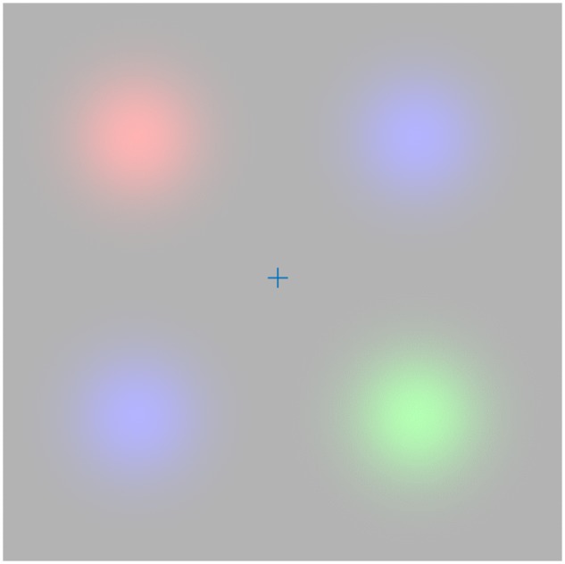
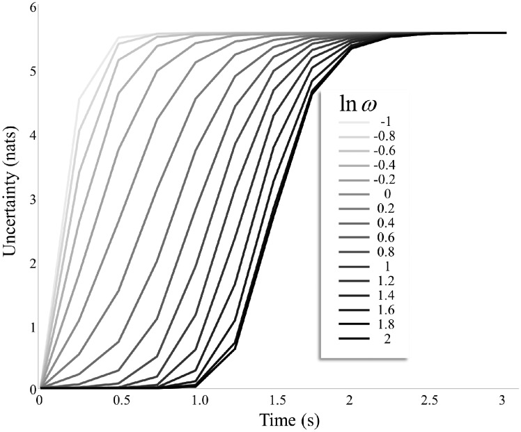
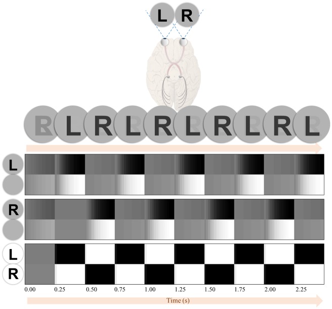
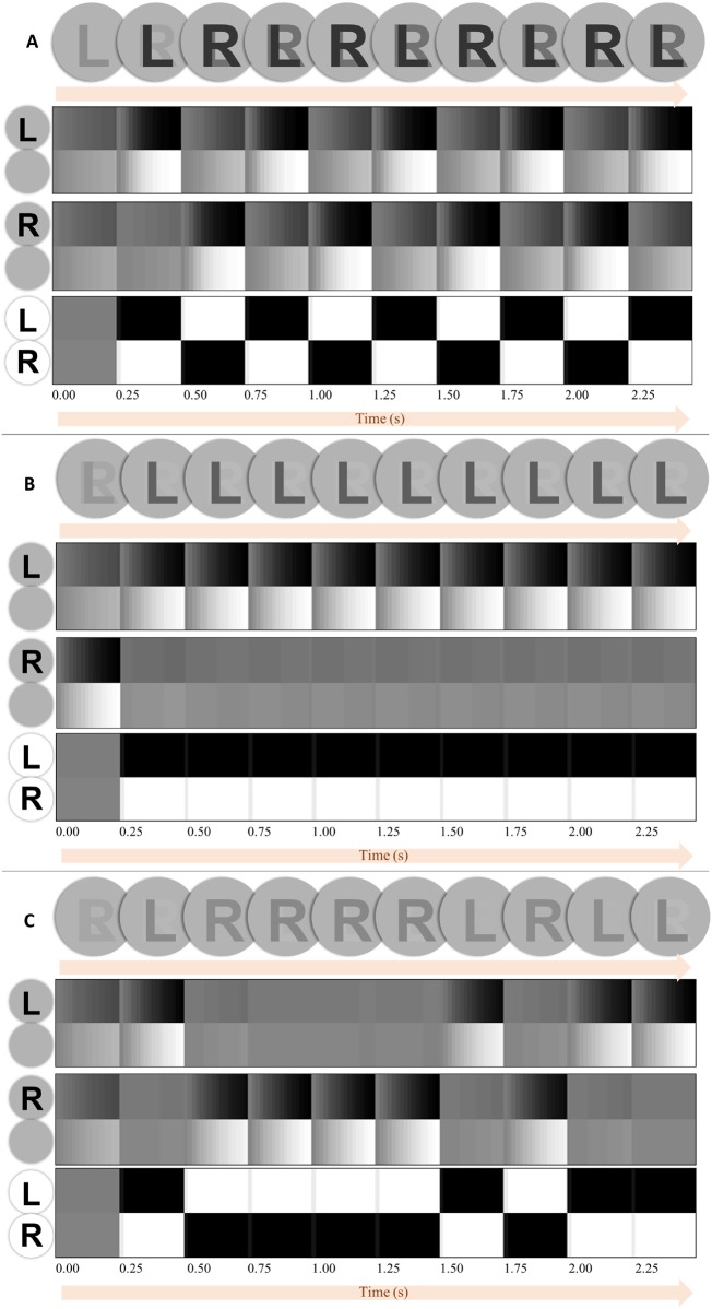
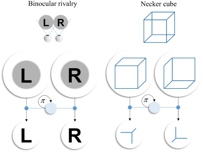
Perceptual awareness depends upon the way in which we engage with our sensorium. This notion is central to active inference, a theoretical framework that treats perception and action as inferential processes. This variational perspective on cognition formalizes the notion of perception as hypothesis testing and treats actions as experiments that are designed (in part) to gather evidence for or against alternative hypotheses. The common treatment of perception and action affords a useful interpretation of certain perceptual phenomena whose active component is often not acknowledged. In this article, we start by considering Troxler fading - the dissipation of a peripheral percept during maintenance of fixation, and its recovery during free (saccadic) exploration. This offers an important example of the failure to maintain a percept without actively interrogating a visual scene. We argue that this may be understood in terms of the accumulation of uncertainty about a hypothesized stimulus when free exploration is disrupted by experimental instructions or pathology. Once we take this view, we can generalize the idea of using bodily (oculomotor) action to resolve uncertainty to include the use of mental (attentional) actions for the same purpose. This affords a useful way to think about binocular rivalry paradigms, in which perceptual changes need not be associated with an overt movement.

Keywords: Bayesian; Troxler fading; active inference; awareness; binocular rivalry.

Figure 1.

Troxler fading. The image shown here is a simple example of the sorts of stimuli used to induce Troxler fading. During free (saccadic) exploration of this image, four blurred circles are visible, in various colours. On fixating on the cross in the centre of this image, the coloured stimuli gradually fade until they match the grey of the background. Once free exploration is resumed, the percepts of the colours are reinstated. This provides an interesting example of the role of action in perception, as the presence or absence of action leads to dramatically different percepts.

Figure 2.

Markov decision process. The schematic above shows a factor graph representation (blue) of a (partially observed) Markov decision process. The circles represent variables, whereas the squares are the factors of the generative model that describe the probabilistic relationship between these variables. The panel on the upper right specifies the form of these relationships. Specifically, A is a probability (likelihood) distribution that specifies the probability of an observation (o) given a hidden state (s). The initial state is given by a probability vector (D), and the subsequent states in the sequence depend upon the probability transition matrix (B). This expresses the dependence of each state on the previous state in the sequence, and upon the policy (course of action) pursued (π). The policy itself is determined by a prior belief that the most probable policies are those that are associated with the lowest expected free energy (G), that itself depends upon prior preference (C). The lower (pink) panels show the Bayesian inversion of the model above, taking the outcomes it generates, and computing posterior beliefs about the states (s), predictive beliefs about future outcomes (o) and beliefs about the policy being pursued (π). These computations are expressed in terms of auxiliary variables playing the role of prediction errors. These are the free energy gradients (ε), and the expected free energy gradients (ς). The transition and likelihood probabilities are each equipped with a superscripted term (ω and ζ, respectively). These represent inverse temperature (or precision) terms that we will use to quantify the (inverse) uncertainty inherent in these probabilities. Note that this Bayesian message passing relies upon local interactions [specifically, marginal message passing (Friston et al. 2017a; Parr et al. 2019)], very much like those between neurons in a network. The notation Cat means a categorical distribution, while σ is a softmax (normalized exponential) function. Note that ω, ζ and C appear in the panels on the right, but do not appear in the factor graph. The reason for this is that the factor graph formalism we have used specifically describes the relationship between random variables (i.e. those things about which we have probabilistic beliefs). Both ω and ζ are parameters of distributions, but we do not model explicit beliefs about them. The influence of C is more subtle. This only has an effect via the expected free energy, so may be thought of as a constituent of the G factor-node.

Figure 3.

Troxler generative model. This schematic illustrates the form of the generative model used to simulate Troxler fading. It includes five hidden state factors representing the colour of the stimulus (shown here in the rows at each corner of the image) at each location and the current fixation location (highlighted in black). The prior probabilities (D) for each hidden state are deterministic, with fixation location starting in the centre, and the colours as indicated above. The only outcome modality is visual (illustrated in the columns below each image), and the mapping from the hidden state associated with a fixated location is shown in the A-matrices here. This is shown for fixation on the lower left (left image) and the lower right (right image). Note that there is only one visual input at any one time, so vision depends upon eye position. The B-matrices specify transitions between hidden states over time. For the stimulus hidden states, these are identity matrices (see upper right). For the fixation location, the transitions depend upon the selected action. Here, we show an example for action four, for which all states transition to state four. This is illustrated explicitly in the transition from the left to the right image. Preferences (C) for each outcome are set to be uniform. Note that this model is formally identical to that pursued in Parr and Friston (2017c) to investigate the salience of different locations under different beliefs about their precisions, but with a different semantic interpretation. The likelihood and transition matrices here are equipped with precision terms to convert them to the probabilities of Figure 2 as follows: ${\mathbf{A}}^{\mathbf{\zeta }}=\sigma (\mathbf{\zeta }\ln (\mathbf{A}+{\mathit{e}}^{-4}))$, ${\mathbf{B}}^{\mathbf{\omega }}=\sigma (\mathbf{\omega }\ln (\mathbf{B}+{\mathit{e}}^{-4}))$. The precision associated with the transition matrix for the control (fixation) state factor is always treated as infinite.

Figure 4.

Simulated Troxler fading. The upper plots illustrate the percepts and saccadic patterns obtained by solving the equations of Figure 2 for the model of Figure 3. The percepts are obtained by weighting the images by their posterior probabilities (which are plotted in the lower plots). (A) It shows the case in which saccadic exploration ensures the maintenance of the image over time. (B) It shows the result of introducing a preference (C-vector Figure 3) for the fixation cross. This results in a failure to explore, and the gradual fading of the percept. (C) It depicts a neglect-syndrome, in which a prior belief that rightward saccades are more probable than leftward saccades gives rise to an asymmetrical exploration, leading to an accumulation of uncertainty about the left side of space. The lower parts of this Figure show the beliefs at each time-point about each of the four stimulus locations. Each plot illustrates beliefs about which stimulus (if any) is present at a given location. From top to bottom, these are upper left, lower left, upper right, lower right. For each of these plots, there are four rows, corresponding to the different hidden states that might be present at those locations. Within these rows, black represents a probability of one that this is the stimulus (hidden state) at this location, whereas white represents a probability of zero. Intermediate shades indicate uncertainty about the hidden state. The red highlights indicate which location is fixated at any given time. For time-steps with no highlight, the fixation cross was fixated.

Figure 5.

Transition precision. This plot illustrates how the time until the images fade depends upon prior beliefs about the precision of transitions. This is expressed as the accumulation of uncertainty over time, where uncertainty is the Shannon entropy summed over posterior beliefs about each stimulus. All lines converge upon maximum uncertainty, corresponding to the completely faded stimuli at the end of row B in Figure 4. As the precision of transitions (ω) is increased, the time it takes for the stimulus to fade increases. This affords an opportunity for empirical investigation, as it suggests the precision of beliefs about transitions (relative to some reference) should be estimable from the time it takes for a percept to fade during fixation of a Troxler stimulus.

Figure 6.

Simulated binocular rivalry. The upper part of this figure shows a simple schematic of a binocular rivalry paradigm. The image presented to each eye is different (here shown simply as an ‘L’ and an ‘R’). This sets up two competing percepts. The row of circles below this shows the posterior beliefs about the stimuli, with the stimulus intensity represented as a monotonic function of its posterior probability. The plots below show beliefs about the presence or absence of the ‘L’, the presence or absence of the ‘R’, and whether attention is directed towards the ‘L’ or ‘R’ features. Note that, when attention is directed towards ‘L’, this induces a belief that the ‘L’ is present, but increases the uncertainty about whether the ‘R’ is present or absent and vice versa. The attended features are consistently those for which the uncertainty was greatest at the previous time-step, just as with the choices of fixation location in the Troxler fading simulation. Although changes in percept coincide with the changes in attentional focus, the two are not equivalent. The former are changes in posterior beliefs, and are consequent upon the changes in precision assumed under alternative attentional choices. The subtlety of this distinction, and the reciprocal causation (attentional choices depend upon posterior beliefs) between the two may underwrite debates about the relationship between attention and awareness, e.g. (Lamme 2003).

Figure 7.

Precisions. This figure shows three special cases of the generative model used above, to provide some intuition as to the behaviour of the simulations. The upper plots (A) show the same set-up as in Fig. 6, with the same generative process giving rise to the data. However, we have adjusted the beliefs of our synthetic subject such that they estimate the precision of transitions to be higher (i.e. a less changeable environment). Although the perceptual switches still continue, the percept does not change as dramatically, as beliefs about the previously attended stimuli persist for a greater time. In the limiting case in which a subject believes the world does not change at all the percept would appear as a mixture of the two stimuli that does not change over time (note that a minority of people do indeed report such fused percepts, but that this leads to their exclusion from standard rivalry studies). In other words, beliefs about the precision of transitions in a person’s generative model may underwrite their susceptibility to rivalry. The middle plots (B) in this figure illustrate the influence of the likelihood precision associated with each stimulus. Here, we have decreased the precision for both stimuli, the ‘R’ stimulus more than the ‘L’ stimulus. This alters the subject’s beliefs about the ‘noisiness’ of the two observations she could make, such that both are noisy, but the ‘L’ stimulus is more reliable. Experimentally, this sort of belief can be induced by changing the contrast of the image presented to each eye. Notably, our subject infers that the best policy is to attend only to the relatively unambiguous ‘L’ stimulus and to consistently ignore the ambiguous ‘R’. The lowest plot (C) shows the same manipulation as (B), but with a much subtler difference between the two precisions. This is just enough to break the symmetry between the two stimuli, but not enough to eliminate perceptual switching. The three examples in this figure illustrate that, even with exactly the same sensory data, different prior beliefs about the generation of these data can lead to dramatically different perceptual inferences. These differences offer the opportunity to investigate the distinct computational phenotypes that underwrite individual differences in perceptual experience.

Figure 8.

Multi-stable perception. The schematic shown above illustrates how the mechanisms we have employed to simulate binocular rivalry may generalize to other forms of multi-stable perception. This uses the Necker cube as an illustrative example but could be applied to other paradigms. On the left, we show the key features of the generative model used for the rivalry simulation. There are two hidden state factors that represent the presence or absence of ‘L’ and of ‘R’. These generate (black vertical arrows) outcomes that are informative about the presence or absence of each of these visual features. The mapping from the states to their respective outcomes may be very precise or imprecise, depending upon the allocation of attention (a third hidden state factor shown in pale blue), which itself depends upon the choice of policy (π). This selects which of the two likelihood mappings is precise. On the right, we illustrate how changing the labels of each of these states and outcomes (without changing the generative model itself) lets us reinterpret the simulation results above in terms of the multi-stable perception associated with a Necker cube. This implies a common architecture for the neuronal message passing, even if implemented in different neuroanatomical structures (Loued-Khenissi et al. 2019).

References

1. Alais D, van Boxtel JJ, Parker A. et al. Attending to auditory signals slows visual alternations in binocular rivalry. Vision Res 2010;50:929–35. - PubMed
1. Alpers GW, Gerdes ABM.. Here is looking at you: emotional faces predominate in binocular rivalry. Emotion 2007;7:495–506. - PubMed
1. Bachy R, Zaidi Q.. Factors governing the speed of color adaptation in foveal versus peripheral vision. J Opt Soc Am A 2014;31:A220–5. - PubMed
1. Bachy R, Zaidi Q.. Troxler fading, eye movements, and retinal ganglion cell properties. Iperception 2014;5:611–2. - PMC - PubMed
1. Bannerman RL, Milders M, De Gelder B. et al. Influence of emotional facial expressions on binocular rivalry. Ophthalmic Physiol Opt 2008;28:317–26. - PubMed