Spatial confidence sets for raw effect size images

Abstract

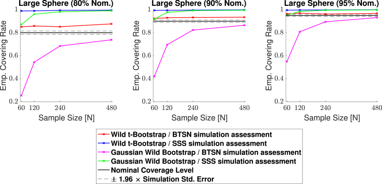
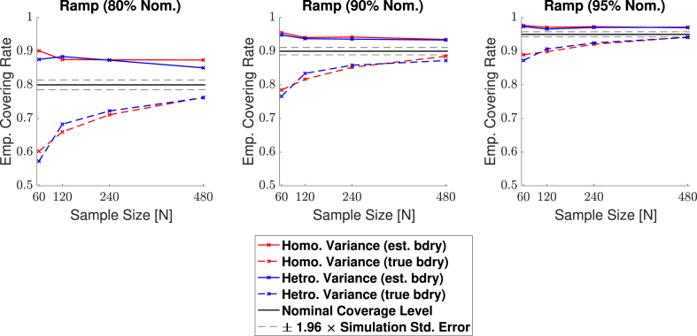
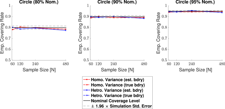
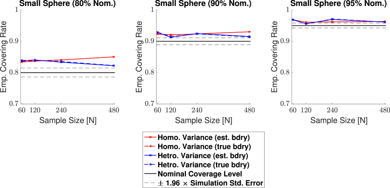
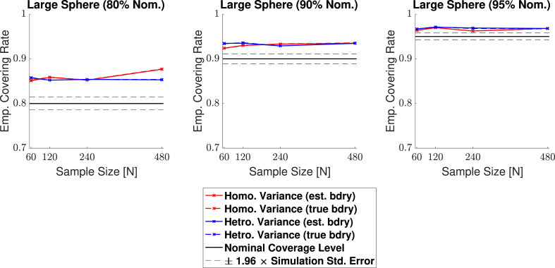
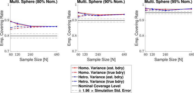
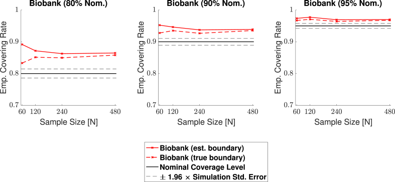
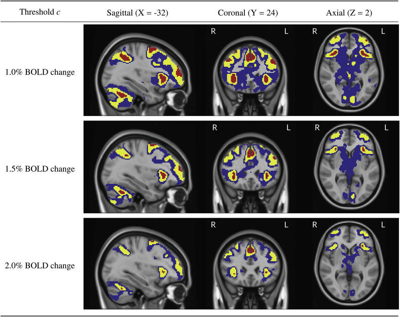
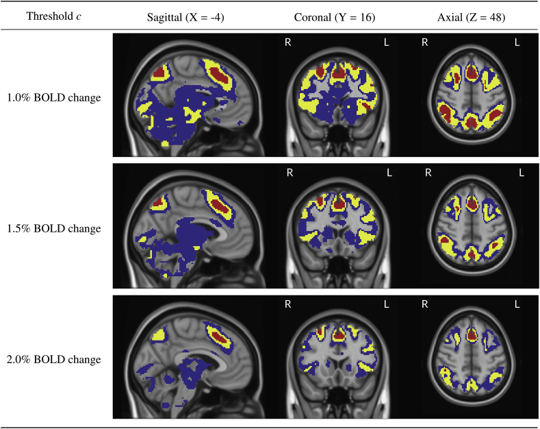
The mass-univariate approach for functional magnetic resonance imaging (fMRI) analysis remains a widely used statistical tool within neuroimaging. However, this method suffers from at least two fundamental limitations: First, with sufficient sample sizes there is high enough statistical power to reject the null hypothesis everywhere, making it difficult if not impossible to localize effects of interest. Second, with any sample size, when cluster-size inference is used a significant p-value only indicates that a cluster is larger than chance. Therefore, no notion of confidence is available to express the size or location of a cluster that could be expected with repeated sampling from the population. In this work, we address these issues by extending on a method proposed by Sommerfeld et al. (2018) (SSS) to develop spatial Confidence Sets (CSs) on clusters found in thresholded raw effect size maps. While hypothesis testing indicates where the null, i.e. a raw effect size of zero, can be rejected, the CSs give statements on the locations where raw effect sizes exceed, and fall short of, a non-zero threshold, providing both an upper and lower CS. While the method can be applied to any mass-univariate general linear model, we motivate the method in the context of blood-oxygen-level-dependent (BOLD) fMRI contrast maps for inference on percentage BOLD change raw effects. We propose several theoretical and practical implementation advancements to the original method formulated in SSS, delivering a procedure with superior performance in sample sizes as low as N=60. We validate the method with 3D Monte Carlo simulations that resemble fMRI data. Finally, we compute CSs for the Human Connectome Project working memory task contrast images, illustrating the brain regions that show a reliable %BOLD change for a given %BOLD threshold.

Graphical abstract

Fig. 1

Schematic of the colour-coded regions used to visually represent the Confidence Sets (CSs) and point estimate set. CSs displayed in the glass brain were obtained by applying the method to 80 participants contrast data from the Human Connectome Project working memory task, using a a $c=2.0\text{\%}$ BOLD change threshold at a confidence level of $1-\alpha =95\text{\%}$.

Fig. 2

A demonstration of how the CSs are computed for a realization of the GLM $\mathit{Y}\left(\mathit{s}\right)=\mathit{X}\mathit{\beta }\left(\mathit{s}\right)+\mathbf{\epsilon }\left(\mathit{s}\right)$ in one dimension, for each location $\mathit{s}$. The yellow voxels ${\hat{\mathcal{A}}}_c$ are obtained by thresholding the observed group contrast map at threshold c; this is the best guess of ${\mathcal{A}}_c$, the set of voxels whose true, noise-free raw effect surpasses c. The red upper CS ${\hat{\mathcal{A}}}_c^{+}$ and blue lower CS ${\hat{\mathcal{A}}}_c^{–}$ are computed by thresholding the signal at $c+k\hat{\sigma }\left(\mathit{s}\right)v_w$ and $c-k\hat{\sigma }\left(\mathit{s}\right)v_w$, respectively. We have $\left(1-\alpha \right)100\text{\%}$ confidence that ${\hat{\mathcal{A}}}_c^{+}\subset {\mathcal{A}}_c\subset {\hat{\mathcal{A}}}_c^{–}$, i.e. that ${\hat{\mathcal{A}}}_c^{+}$ (red) is completely within the true ${\mathcal{A}}_c$, and ${\mathcal{A}}_c$ is completely within ${\hat{\mathcal{A}}}_c^{-}$ (blue). We find the critical value k from the $\left(1-\alpha \right)100$ percentile of the maximum distribution of the absolute error process over the estimated boundary $\partial {\hat{\mathcal{A}}}_c$ (green $•$’s) using the Wild t-Bootstrap; $\hat{\sigma }$ is the estimated standard deviation and $v_w$ is the normalised contrast variance.

Fig. 3

Demonstrating the resolution issue for testing the subset condition ${\hat{\mathcal{A}}}_c^{+}\subset {\mathcal{A}}_c\subset {\hat{\mathcal{A}}}_c^{–}$. Fig. 3a: Here ${\mathcal{A}}_c$ is comprised of the right half of the image (all green and yellow pixels), and ${\hat{\mathcal{A}}}_c^{+}$ is shown as yellow pixels. It appears that ${\hat{\mathcal{A}}}_c^{+}\subset {\mathcal{A}}_c$. Fig. 3b: The same configuration as Fig. 3a at double the resolution. Here, we have enough detail to see that ${\hat{\mathcal{A}}}_c^{+}$ has crossed the boundary $\partial {\mathcal{A}}_c$ (yellow seeping into blue), and the subset condition ${\hat{\mathcal{A}}}_c^{+}\subset {\mathcal{A}}_c$ has been violated.

Fig. 4

Linear ramp and circular signals $\mu \left(\mathit{s}\right)$. Fig. 4a: Signal 1. A linear ramp signal that increases from magnitude of 1–3 in the x-direction. Fig. 4b: Signal 2. A circular signal with magnitude of 3 and radius of 30, centred within the region and convolved with a 3 voxel FWHM Gaussian kernel.

Fig. 5

Stationary and non-stationary standard deviation fields of the noise ${\mathrm{\epsilon }}_i\left(\mathit{s}\right)$. Fig. 5a: Standard Deviation 1. Stationary variance of 1 across the region. Fig. 5b: Standard Deviation 2. Non-stationary (linear ramp) standard deviation field increasing from $\sqrt{0.5}$ to $\sqrt{1.5}$ in the y-direction.

Fig. 6

The four 3D signal types $\mu \left(\mathit{s}\right)$, from top-to-bottom: small sphere, large sphere, multiple spheres, and the UK Biobank full mean image. Note that the colormap limits for the first three signal types are from 0 to 3, while the colormap limits for the UK Biobank mean image is from −0.4 to 0.5.

Fig. 7

Coverage results for the 2D circular signal simulation with homogeneous Gaussian noise (Signal 2., Standard deviation 1. in Fig. 5). Empirical coverage results are presented for implementations of the CS method with and without the Wild t-Bootstrap we propose in Section 2.2 and the interpolation schema for assessing simulations results we propose in Section 2.4. All empirical coverage results for simulations using the SSS assessment method are close to 100%, suggesting that this assessment substantially biases the results upwards. Using our proposed assessment method, while both the Wild t-Bootstrap and Gaussian Wild bootstrap converge to the nominal level, the Wild t-Bootstrap performed better for small sample sizes.

Fig. 8

Coverage results for the 3D large spherical signal (Signal 2. in Fig. 6) simulation with homogeneous Gaussian noise. Empirical coverage results are presented for implementations of the CS method with and without the Wild t-Bootstrap we propose in Section 2.2, and the interpolation schema for assessing simulations results we propose in Section 2.4. Once again, all simulations using the SSS assessment method quickly converge to close to 100%. Using our proposed assessment method, the Gaussian Wild bootstrap had severe under-coverage for small sample sizes, while the Wild t-Bootstrap results hover slightly above the nominal level for all sample sizes.

Fig. 9

Coverage results for Signal 1., the 2D linear ramp signal. While the true boundary coverage results (dashed curves) fall under the nominal level, results for the estimated boundary method (solid curves) that must be applied to real data remain above the nominal level. Performance of the method improved for larger confidence levels, and in particular, the estimated boundary results for a 95% confidence level seen in the right plot hover slightly above nominal coverage for all sample sizes.

Fig. 10

Coverage results for Signal 2., the 2D circular signal. Coverage performance was close to nominal level in all simulations. The method was robust as to whether the subject-level noise had homogeneous (red curves) or heterogeneous variance (blue curves), or as to whether the estimated boundary (dashed curves) or true boundary (solid curves) method was used; in all plots, all of the curves lie practically on top of each other.

Fig. 11

Coverage results for Signal 1., the 3D small spherical signal. For all confidence levels, coverage remained above the nominal level in all simulations, and for a 95% confidence level (right plot), coverage hovered slightly above the nominal level for all sample sizes. The method was robust as to whether the subject-level noise had homogeneous (red curves) or heterogeneous variance (blue curves), or as to whether the estimated boundary (dashed curves) or true boundary (solid curves) method was used.

Fig. 12

Coverage results for Signal 2., the large 3D spherical signal. Coverage results here were very similar to the results for the small spherical signal shown in Fig. 11, suggesting that the method is robust to changes in boundary length.

Fig. 13

Coverage results for Signal 3., the multiple spheres signal. Once again, for all confidence levels, coverage remained above the nominal level in all simulations. Here, the true boundary method (dashed curves) performed slightly better than the estimated boundary method (solid curves) in small sample sizes, although the choice of boundary made less of a difference for a higher confidence level. For a 95% confidence level (right plot), all results hover slightly above nominal coverage for all sample sizes.

Fig. 14

Coverage results for Signal 4., the UK Biobank full mean signal, where the full standard deviation image was used as the standard deviation of the subject-level noise fields. Coverage results here were similar to the results for the multiple spheres signal shown in Fig. 13; in small sample sizes, coverage was slightly improved for the true boundary method (dashed curves) compared to the estimated boundary method (solid curves), however, for a 95% confidence level (right plots), all results hover slightly above nominal coverage for all sample sizes.

Fig. 15

Slice views of the Confidence Sets for 80 subjects data from the HCP working memory task for $c=1.0\text{\%},1.5\text{\%}$ and $2.0\text{\%}$ BOLD change thresholds. The upper CS ${\hat{\mathcal{A}}}_c^{+}$ is displayed in red, and the lower CS ${\hat{\mathcal{A}}}_c^{–}$ displayed in blue. In yellow is the point estimate set ${\hat{\mathcal{A}}}_c$, the best guess from the data of voxels that surpassed the BOLD change threshold. The red upper CS has localized regions in the frontal gyrus, frontal pole, anterior insula, supramarginal gyrus and cerebellum for which we can assert with $95\text{\%}$ confidence that there has been (at least) a $1.0\text{\%}$ BOLD change raw effect.

Fig. 16

Further slice views of the Confidence Sets. Here, we see that the red upper CS has also localized regions in the anterior cingulate, superior front gyrus, supramarginal gyrus, and precuneous for which we can assert with $95\text{\%}$ confidence that there has been (at least) a $1.0\text{\%}$ BOLD change raw effect.

References

1. Hariri Ahmad R., Tessitore Alessandro, Mattay Venkata S., Fera Francesco, Weinberger Daniel R. The amygdala response to emotional stimuli: a comparison of faces and scenes. Neuroimage. September 2002;17(1):317–323. - PubMed
1. Alfaro-Almagro Fidel, Jenkinson Mark, Bangerter Neal K., Andersson Jesper L.R., Griffanti Ludovica, Douaud Gwenaëlle, Sotiropoulos Stamatios N., Jbabdi Saad, Hernandez-Fernandez Moises, Vallee Emmanuel, Vidaurre Diego, Webster Matthew, McCarthy Paul, Rorden Christopher, Daducci Alessandro, Alexander Daniel C., Zhang Hui, Dragonu Iulius, Matthews Paul M., Miller Karla L., Smith Stephen M. Image processing and quality control for the first 10,000 brain imaging datasets from UK biobank. Neuroimage. February 2018;166:400–424. - PMC - PubMed
1. Barch Deanna M., Burgess Gregory C., Harms Michael P., Petersen Steven E., Schlaggar Bradley L., Corbetta Maurizio, Glasser Matthew F., Curtiss Sandra, Dixit Sachin, Feldt Cindy, Nolan Dan, Bryant Edward, Tucker Hartley, Owen Footer, Bjork James M., Poldrack Russ, Smith Steve, Johansen-Berg Heidi, Snyder Abraham Z., Van Essen David C., WU-Minn HCP Consortium Function in the human connectome: task-fMRI and individual differences in behavior. Neuroimage. October 2013;80:169–189. - PMC - PubMed
1. Chen Gang, Taylor Paul A., Cox Robert W. Is the statistic value all we should care about in neuroimaging? Neuroimage. February 2017;147:952–959. - PMC - PubMed
1. Chernozhukov Victor, Chetverikov Denis, Kato Kengo. 2013. Gaussian Approximations and Multiplier Bootstrap for Maxima of Sums of High-Dimensional Random Vectors.
Publication types