Benchmarking Parametric and Machine Learning Models for Genomic Prediction of Complex Traits

Abstract

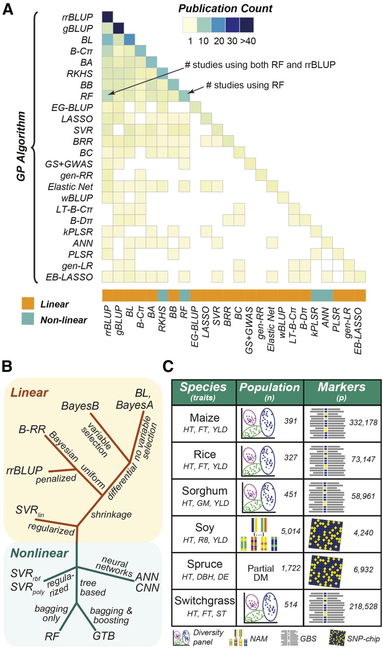
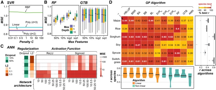
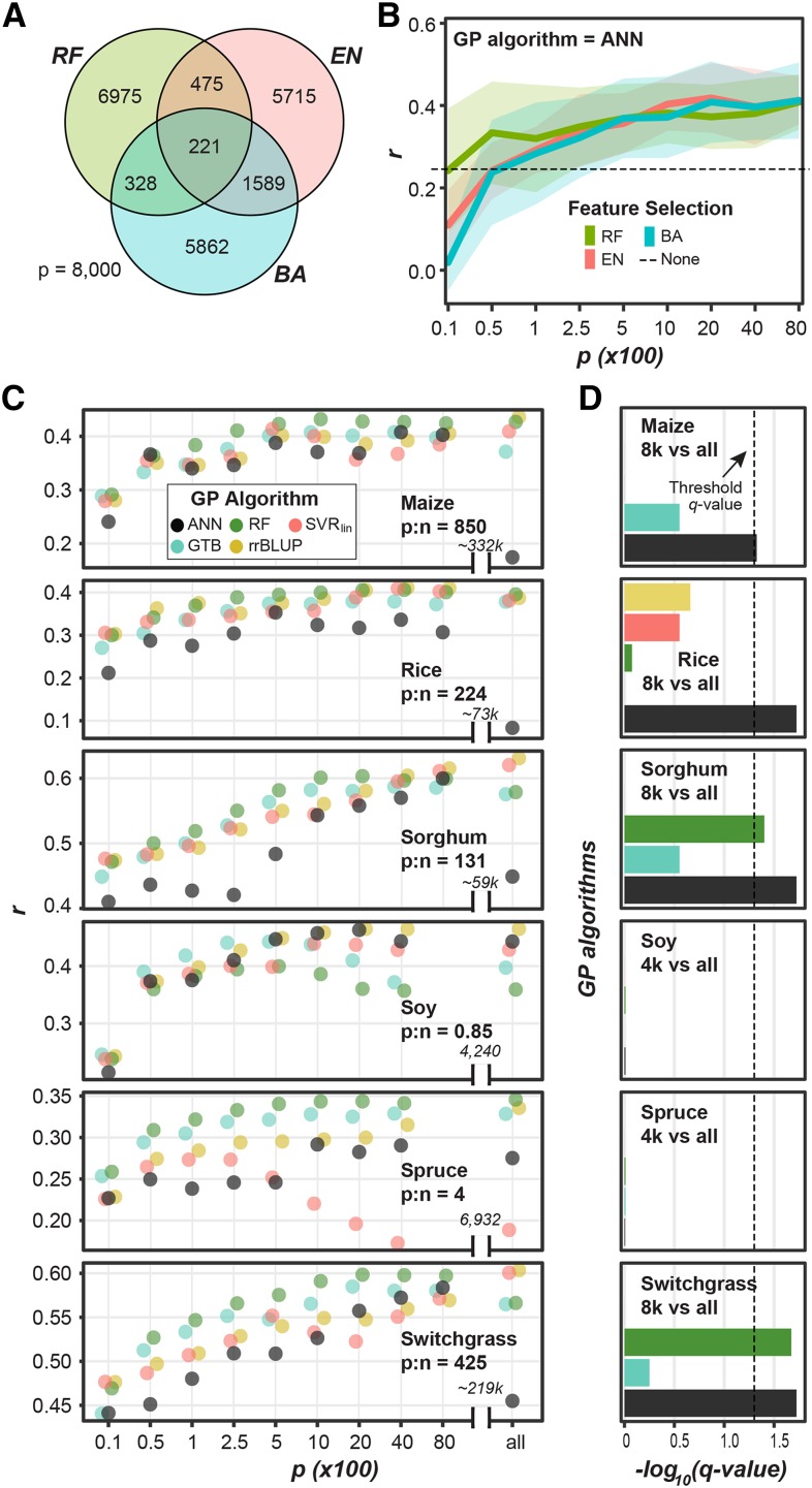
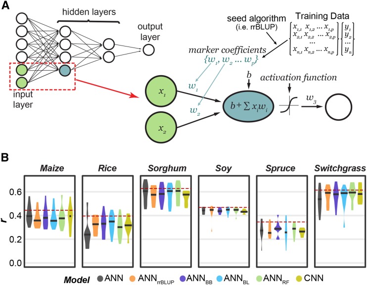
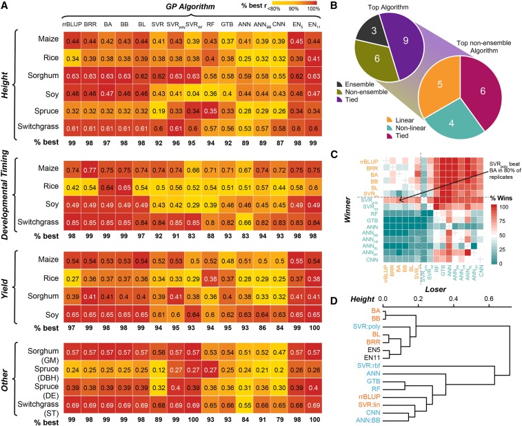
The usefulness of genomic prediction in crop and livestock breeding programs has prompted efforts to develop new and improved genomic prediction algorithms, such as artificial neural networks and gradient tree boosting. However, the performance of these algorithms has not been compared in a systematic manner using a wide range of datasets and models. Using data of 18 traits across six plant species with different marker densities and training population sizes, we compared the performance of six linear and six non-linear algorithms. First, we found that hyperparameter selection was necessary for all non-linear algorithms and that feature selection prior to model training was critical for artificial neural networks when the markers greatly outnumbered the number of training lines. Across all species and trait combinations, no one algorithm performed best, however predictions based on a combination of results from multiple algorithms (i.e., ensemble predictions) performed consistently well. While linear and non-linear algorithms performed best for a similar number of traits, the performance of non-linear algorithms vary more between traits. Although artificial neural networks did not perform best for any trait, we identified strategies (i.e., feature selection, seeded starting weights) that boosted their performance to near the level of other algorithms. Our results highlight the importance of algorithm selection for the prediction of trait values.

Keywords: GenPred; Genomic Prediction; Genomic selection; Shared Data Resources; artificial neural network; genotype-to-phenotype.

Figure 1

Algorithms used and compared in past GP studies and algorithms and data included in the GP benchmark. (A) Number of times a GP algorithm was utilized (diagonal) or directly compared to other GP algorithms (lower triangle) out of 91 publications published between 2012-2018 (Table S1). GP algorithms were included if they were utilized in >1 study. (B) A graphical representation of the GP algorithms included in the study and their relationship to each other. Colors designate if the algorithm identifies only linear (orange) or linear and non-linear (green) relationships. The placement of each algorithm on the tree designates (qualitatively) the relationship between different algorithms. The labels at each branch provide more information about how algorithms in that branch differ from others. rrBLUP, ridge regression Best Linear Unbiased Predictor; BRR, Bayesian Ridge Regression; BA, BayesA; BB, BayesB; BL, Bayesian LASSO; SVR, Support Vector Regression (kernel type: lin, linear; poly, polynomial; rbf, radial basis function); RF, Random Forest; GTB, Gradient Tree Boosting; ANN, Artificial Neural Network; CNN, Convolutional Neural Network. (C) Species and traits included in the benchmark with training population types and sizes and marker types and numbers for each dataset. NAM: Nested Association Mapping. DM: partial diallel mating. GBS: genotyping by sequencing. SNP: single nucleotide polymorphism. HT: height. FT: flowering time. YLD: yield. GM: grain moisture. R8: time to R8 developmental stage. DBH: diameter at breast height. DE: wood density. ST: standability.

Figure 2

Grid search results for height in maize and overall GP algorithm performance for predicting height across species. (A) Average of mean squared error (MSE) over hyperparameter space (penalty, C) for Support Vector Regression (SVR) based models predicting height in maize. SVR_rbf and SVR_poly results are shown using gamma = 1x10⁻⁵ and 1x10⁻⁴, respectively. Poly: polynomial. RBF: Radial Basis Function. (B) Distribution of MSEs across hyperparameter space for Random Forest (RF; left) and Gradient Tree Boosting (GTB; right) as the maximum features available to each tree (Max Features) and maximum tree depth (color) change. GTB results are shown using a learning rate = 0.01. (C) Average MSE across hyperparameter space for ANN models with different network architectures, degrees of regularization (dropout or L2), using either the Rectified Linear Unit (ReLU; left) or Sigmoid (right) activation function. (D) Mean performance (Pearson’s Correlation Coefficient: r, text) for predicting height and percent best r (colored box, top algorithm for each species = 100% (red)). White text: the best r values. Violin-plots show the median and distribution of r values for each trait (right) and algorithm (bottom).

Figure 3

Impact of feature selection on GP algorithm performance. (A) Average number of overlapping markers in the top 8,000 markers selected by three feature selection algorithms for predicting height in maize across ten replicates. EN: Elastic Net. (B) Change in ANN predictive performance (r) at predicting height in maize as the number of input markers (p) selected by three feature selection algorithms (BayesA: BA, EN, and Random Forest: RF) increases. Dashed line: mean r when all 332,178 maize markers were used. (C) Mean r of rrBLUP, SVR_lin, RF, GTB, and ANN models for predicting height using subsets or all (X-axis) markers as features across 10 replicate feature selection and ML runs for each of six species with their ratios of numbers of markers (p) to numbers of lines (n) shown. Data points were jittered horizontally for ease of visualization. (D) The significance (-log₁₀(q-value), paired Wilcoxon Signed-Rank test) of the difference in r between models from different GP algorithms (colored as in Figure 3C) generated using a subset of 4,000 or 8,000 and all markers as input. Dotted line designates significant differences (p-value < 0.05).

Figure 4

Description and performance results of the seeded ANN approach. (A) An overview of the seeded ANN approach. The network in the top left is an example of a fully connected ANN with 6 input nodes (i.e., 6 markers), two hidden layers, and one output layer (i.e., predicted trait value). The blue node in the first hidden layer represents an example node that will have seeded weights. For this node, the weights (w) connecting each input node to the hidden node will be seeded from the coefficient/importance for each marker as determined by another GP algorithm using the training data. b: bias, which helps control the value at which the activation function will trigger. (B) The distribution of model performance (r) using only all random (None) or 25% seeded (rrBLUP, BayesB, BL, RF) weight initialization, and convolutional neural networks (CNNs). The mean performance of the overall top performing algorithm (i.e., not necessary ANN) shown as dotted red line.

Figure 5

Comparison of algorithms for predicting additional traits. (A) Mean model performance (r; text) for each species/trait combination (y-axis) for each GP algorithm (x-axis). White text: r of the best performing algorithm(s) for a species. Colored boxes: percent of best performance (r) for a species, with the top algorithm for each species = 100% (red). The median % of best performance for each GP algorithm for each type of trait (i.e., height, developmental timing, yield, other) is shown below each heatmap. GM: sorghum grain moisture. DBH and DE: diameter at breast height and wood density, respectively, for spruce. ST: standability for switchgrass. (B) Top left: summary of the number of species/trait combinations that were predicted best by an ensemble (gray) or a non-ensemble model (yellow), or predicted equally well by both (purple). Bottom right: among non-ensemble models that performed or tied for the best, the number of species/trait combinations that were predicted best by a linear (blue) or a non-linear model (green) or predicted equally well by both (orange). (C) Percent of replicates where one GP algorithm (y-axis, winner) outperformed another GP algorithm (x-axis, loser) for predicting height in switchgrass. Orange and cyan texts: linear and non-linear algorithms, respectively. (D) Hierarchical clustering of GP algorithms based on mean predictive performance across all species/trait combinations. Algorithm colored as in (C).

References

1. Angermueller C., Pärnamaa T., Parts L., and Stegle O., 2016. Deep learning for computational biology. Mol. Syst. Biol. 12: 878 10.15252/msb.20156651 - DOI - PMC - PubMed
1. Beaulieu J., Doerksen T. K., MacKay J., Rainville A., and Bousquet J., 2014. Genomic selection accuracies within and between environments and small breeding groups in white spruce. BMC Genomics 15: 1048 10.1186/1471-2164-15-1048 - DOI - PMC - PubMed
1. Bellot P., de los Campos G., and Pérez-Enciso M., 2018 Can Deep Learning Improve Genomic Prediction of Complex Human Traits? Genetics genetics.2018. - PMC - PubMed
1. Benjamini Y., and Hochberg Y., 1995. Controlling the False Discovery Rate: A Practical and Powerful Approach to Multiple Testing. J R Stat Soc Ser. B Stat Methodol 57: 289–300.
1. Bermingham, M. L., R. Pong-Wong, A. Spiliopoulou, C. Hayward, I. Rudan et al., 2015 Application of high-dimensional feature selection: evaluation for genomic prediction in man. Sci. Rep. 1–12. 10.1038/srep10312 - DOI - PMC - PubMed
Publication types