Dimensions of control for subthreshold oscillations and spontaneous firing in dopamine neurons

Abstract

Dopaminergic neurons (DAs) of the rodent substantia nigra pars compacta (SNc) display varied electrophysiological properties in vitro. Despite this, projection patterns and functional inputs from DAs to other structures are conserved, so in vivo delivery of consistent, well-timed dopamine modulation to downstream circuits must be coordinated. Here we show robust coordination by linear parameter controllers, discovered through powerful mathematical analyses of data and models, and from which consistent control of DA subthreshold oscillations (STOs) and spontaneous firing emerges. These units of control represent coordinated intracellular variables, sufficient to regulate complex cellular properties with radical simplicity. Using an evolutionary algorithm and dimensionality reduction, we discovered metaparameters, which when regressed against STO features, revealed a 2-dimensional control plane for the neuron's 22-dimensional parameter space that fully maps the natural range of DA subthreshold electrophysiology. This plane provided a basis for spiking currents to reproduce a large range of the naturally occurring spontaneous firing characteristics of SNc DAs. From it we easily produced a unique population of models, derived using unbiased parameter search, that show good generalization to channel blockade and compensatory intracellular mechanisms. From this population of models, we then discovered low-dimensional controllers for regulating spontaneous firing properties, and gain insight into how currents active in different voltage regimes interact to produce the emergent activity of SNc DAs. Our methods therefore reveal simple regulators of neuronal function lurking in the complexity of combined ion channel dynamics.

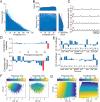
Fig 1. Error function description and test optimization results.

(A) The traditional transfer function from normalized feature value to error value. The error value is the number of experimentally observed standard deviations from the experimentally observed mean for the model generated feature value. This method targets one ‘best’ feature value at the observed mean (function minimum). (B) Soft-thresholded error, where a number of standard deviations (in this case 2) is permitted to give equivalent error by reducing error to zero within that region. This approach considers any model within an observed range as equally plausible. (C) The decision making value when ranks are equal in the NSDE algorithm is crowdedness in feature space. Models with lower crowdedness (e.g. in the blue box) are preferred over models with higher crowdedness (e.g. in the red box). This promotes diversity of model activity and fills the full range of experimentally observed activity. (D) Sigmoidal transfer functions converting parameter values (x-axis) to feature values (y-axis) for the test optimizations. Solid lines show transfer functions for parameter 1 into feature 1; the dotted line shows transfer function for parameter 2 into feature 2 in one optimization (orange). In the other two optimizations feature 2 is calculated from a sigmoidal transfer function on either (P1 − P2) × 2 (green), or (P1 + P2)/2 (purple). (E) Test optimization result. Models shown in feature space are approximately uniformly distributed regardless of location of transfer function in parameter space. Curves at top and right in (E) and (F) are based on histograms with 100 bins. (F) Test optimization result. All model parameter sets plotted in the 2D parameter space. Distributions are Gaussian, with mean and standard deviation dependent on center and slope of the sigmoidal transfer function shown in (D).

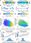
Fig 2. Population-based evolutionary search found models covering the range of target features.

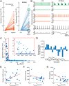
(A) STO frequency and amplitude for every parameter set simulated during the optimization. Red rectangle indicates target feature values. (B) View of red rectangle in (A) representing ‘good’ models. Histograms show distribution of values for each feature. Red lines represent uniform distribution at mean count. (C) Examples of model membrane potential during STOs with different feature values. (D) Correlation coefficients for STO features with PC scores. Red bars indicate highest correlated PC. (E) Parameter coefficients of PCs most highly correlated with STO features. (F) STO amplitude (left) and frequency (right) for models, shown in space of score for PC 19 (x-axis) and PC 22 (y-axis). Each square shows mean feature value for all models found within that segment of parameter space. Blank space indicates no models were found for that parameter combination. Models were found using 22 independently varying parameters. (G) As in (F), but showing models found during the 2-dimensional optimization using PC 19 and PC 22 as metaparameters controlling the 22 parameters according to the coefficients shown in (E).

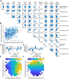
Fig 3. PLSR identified predictors of features.

(A) Parameter coefficients from PLSR against STO frequency and amplitude. Rows indicate PLSR performed on output parameter sets from 5 independent trials of the optimization algorithm using different random seeds. (B) Mean coefficient from the 5 trials for each parameter. Error bars (not visible due to small size) show standard deviation. (C) STO frequency for models shown in the space of predicted amplitude and frequency for that parameter set, according to the PLSR coefficients. Color shows mean STO frequency for all models within a particular bin of predicted frequency and amplitude space. Empty squares indicate no models in that range of predicted feature space. (D) As in (C), but with color showing model STO amplitude. (E) All models sorted by predicted feature values according to PLSR coefficients, and binned into 10 equal-width bins of predicted STO feature values. Boxplots show actual feature values of all models in that bin. Centre line shows median, box shows interquartile range, and whiskers show range. Red lines across boxplots show best fitting sigmoid functions calculated using least squares error. Outside histograms show distribution of predicted STO feature values (horizontal) and actual STO feature values (vertical). Red lines in horizontal histograms show Gaussian fits of models in parameter space, as in Fig 2E. Red lines in vertical histograms show uniform distribution at mean count.

Fig 4. Spiking optimization features.

(A) Scatter plots of feature pairs for all 727 models present in the final population. Red lines show correlations with coefficients above 0.25. (B) Zoom on STO frequency vs. spontaneous FR. Colored circles correspond to colored traces in Fig 5. (C) PLSR coefficients for spontaneous FR. (D) PLSR coefficients for AHP depth. (E) Spontaneous FR for models shown in the space of predicted spontaneous FR (x-axis) and AHP depth (y-axis) for each parameter set, according to the PLSR coefficients. Color shows mean spontaneous FR for all models within a particular bin of predicted FR and AHP depth. Empty squares indicate no models in that range of predicted feature space. (F) As in (E), but with color showing model AHP depth.

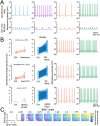
Fig 5. Spiking model channel perturbation results.

(A) Spontaneous firing and STO voltage traces from 4 example parameter sets. Colored traces correspond to models circled in Fig 4B. (B) Effect of blocking potassium currents on spontaneous firing frequencies. Left plots with orange points are recreated from Figure 3C of [64] (BK Block), Figure 2D of [24] (KA Block), and Figure 1F of [10] (KERG Block). Right plots with blue points show effects in all good models. Points paired by lines indicate each model. Traces correspond to the orange and green models shown in (A), for each of the channel block conditions. (C) Effect of positive and negative scaling of depolarizing conductances (NaT, CaL and HCN) on spontaneous firing frequency. Each square shows a different scaling factor applied to ${\overline{g}}_{\text{NaT}}$, with 9 scaling factors ranging from 0 to 2 applied to all 727 good models. Within each square, x-axis shows scaling of ${\overline{g}}_{\text{CaL}}$ and y-axis shows scaling of ${\overline{g}}_{\text{HCN}}$. Colors indicate mean change in frequency from default value for all 727 models.

Fig 6. Burst susceptibility of models under SK block.

(A) CV ISI during normal spontaneous firing (Ctrl) and with SK conductance reduced to 0 (SK Block). Left plot with orange points is approximated from Figure 2A of [32]. Right plot with blue points shows the population of models. Black, orange and green circles indicate CV ISI values of traces shown in (B). (B) Example voltage traces for spontaneous firing (top) and STO (bottom) in the normal (Ctrl) and SK Block conditions, for parameter sets demonstrating 3 behaviors: large increase (green), small increase (orange) and no change (black) to CV ISI under SK Block. (C) Kv2 conductance (x-axis) vs. spontaneous firing CV ISI (y-axis). Inset shows zoom in on red boxed region (low ${\overline{g}}_{\text{Kv2}}$). (D) PLSR coefficients for CV ISI for all parameter sets with ${\overline{g}}_{\text{Kv2}}<0.005$. (E-G) Scatter plots of 22 models in which all burst characteristics could be calculated, showing highest correlated parameter (x-axes) with each burst characteristic (y-axes). Each point is a parameter set.

Fig 7. Spontaneous firing and STO interaction.

(A) Phase plane of membrane potential for spontaneous firing (blue) and STO (orange) for one model with similar frequencies in both regimes. (B) Zoom in on black boxed region of (A). Arrow shows point of crossing at which membrane potential and rate of membrane potential change are identical in both regimes. (C) Voltage traces for spontaneous firing (blue), STO (orange), and STO with spiking currents (NaT, Kv2, BK) activated at point of identical voltage (green). Arrow indicates the point at which spiking currents are activated in the green trace, and the orange and green traces diverge. (D) Phase plane of membrane potential for spontaneous firing (blue), STO plus activated spiking currents (green), and STO plus activated spiking currents plus fractional addition of the state variable difference vector (shades of red). Colors correspond to the key shown to the left. (E) Zoom in on the black boxed region of (D). (F) Interspike intervals for the first 7 ISIs calculated from the first 8 spike times after spiking current activation. (G) Voltage traces for spontaneous firing (blue), STO (orange), and spontaneous firing with spiking currents (NaT, Kv2, BK) deactivated at point of identical voltage (green). Arrow indicates the point at which spiking currents are deactivated in the green trace, and the blue and green traces diverge. (H) Interpeak intervals for the first 19 interpeak intervals calculated from the first 20 oscillation peak times after spiking current deactivation. Colors correspond to the key shown in (F).

References

1. Schultz W. (1998). Predictive reward signal of dopamine neurons. Journal of Neurophysiology, 80(1):1–27. 10.1152/jn.1998.80.1.1 - DOI - PubMed
1. Grace A. A. (2016). Dysregulation of the dopamine system in the pathophysiology of schizophrenia and depression. Nature Reviews Neuroscience, 17:524–532. 10.1038/nrn.2016.57 - DOI - PMC - PubMed
1. Khaliq Z. M. and Bean B. P. (2008). Dynamic, nonlinear feedback regulation of slow pacemaking by A-type potassium current in ventral tegmental area neurons. The Journal of Neuroscience, 28(43):10905–10917. 10.1523/JNEUROSCI.2237-08.2008 - DOI - PMC - PubMed
1. Tarfa R. A., Evans R. C., and Khaliq Z. M. (2017). Enhanced sensitivity to hyperpolarizing inhibition in mesoaccumbal relative to nigrostriatal dopamine neuron subpopulations. The Journal of Neuroscience, 37:3311–3330. 10.1523/JNEUROSCI.2969-16.2017 - DOI - PMC - PubMed
1. Neuhoff H., Neu A., Liss B., and Roeper J. (2002). Ih channels contribute to the different functional properties of identified dopaminergic subpopulations in the midbrain. The Journal of Neuroscience, 22(4):1290–1302. 10.1523/JNEUROSCI.22-04-01290.2002 - DOI - PMC - PubMed
Publication types