The Benefit of Slice Timing Correction in Common fMRI Preprocessing Pipelines

Abstract

Due to the nature of fMRI acquisition protocols, slices cannot be acquired simultaneously, and as a result, are temporally misaligned from each other. To correct from this misalignment, preprocessing pipelines often incorporate slice timing correction (STC). However, evaluating the benefits of STC is challenging because it (1) is dependent on slice acquisition parameters, (2) interacts with head movement in a non-linear fashion, and (3) significantly changes with other preprocessing steps, fMRI experimental design, and fMRI acquisition parameters. Presently, the interaction of STC with various scan conditions has not been extensively examined. Here, we examine the effect of STC when it is applied with various other preprocessing steps such as motion correction (MC), motion parameter residualization (MPR), and spatial smoothing. Using 180 simulated and 30 real fMRI data, we quantitatively demonstrate that the optimal order in which STC should be applied depends on interleave parameters and motion level. We also demonstrate the benefit STC on sub-second-TR scans and for functional connectivity analysis. We conclude that STC is a critical part of the preprocessing pipeline that can be extremely beneficial for fMRI processing. However, its effectiveness interacts with other preprocessing steps and with other scan parameters and conditions which may obscure its significant importance in the fMRI processing pipeline.

Keywords: fMRI — functional magnetic resonance imaging; interleaved 2D multislice sequence; motion correction; preprocessing algorithms; slice timing correction.

FIGURE 1

Visualization of spatial ROI’s used in analysis. Spatial maps for ROI’s used in (A) simulated data, which was identical for each simulated subject, and (B) Real data, in which the ROI varied slightly from subject to subject due to individual subject morphometry.

FIGURE 2

A flowchart of the processing pipeline for real data. (A) A default group level GLM is run on all subjects to obtain a region of activation, which is binarized into a mask and transformed back into each subject’s native space. This mask is used as an ROI to examine t-statistics from five different processing pipelines: (B) No STC, but the data is temporally lowpass filtered, and slice-dependent regressors shifted to account for the acquisition offset are used. (C) Our in house FS STC method is used. (D) FSL STC is used. (E) SPM STC is used. (F) No STC is used, and regressors are not shifted to account for slice offset. The statistics from pipeline b are used to identify 20 voxels with the highest t-statistics in the ROI. The standardized beta values from these 20 voxels are then extracted from the other pipelines, and the values are compared in a pairwise t-test.

FIGURE 3

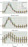
The effect of STC on the accuracy of BOLD response. Normalized HRF’s extracted from the top 20 voxels identified using the shifted regressor method for low, medium, and high motion in simulated data. HRF’s were extracted using FIR deconvolution for each STC method (dashed lines). The reference HRF used in the simulation is plotted as a solid blue line. For each motion level and STC method, HRF’s are combined across all pipeline orders.

FIGURE 4

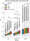
Quantification of BOLD HRF extraction error. SSE of normalized HRF’s deconvolved from STC data, compared to the canonical HRF used in the simulation for low, medium, and high motion. For each motion level and STC method, HRF SSE’s are combined across all pipeline orders.

FIGURE 5

Effect of the order in which STC and MC are applied in the preprocessing pipeline in real data. z-scores from the top 20 voxels from a visual ROI of 30 real subjects’ time series using different preprocessing pipelines, with no smoothing. FS, FSL, and SPM slice timing correction were applied before motion correction, after motion correction, or without any motion correction. For the “Uncorrected” case, only motion correction was applied in the preprocessing pipeline. ‘<’ and ‘>’ Symbols indicate which mean is greater for cases that are not easily distinguishable.

FIGURE 6

The similarity of the selected voxels in our evaluations of simulated data. Dice overlap in simulated data of top 20 voxels for each STC in various pipelines, compared to the top 20 voxels of the shifted regressor method within that pipeline. Uncorrected data in the “No MC” column refers to data that has had no MC or STC.

FIGURE 7

The similarity of the selected voxels in our evaluations of real data, Dice overlap in real data of top 20 voxels for each STC in various pipelines, compared to the top 20 voxels of the shifted regressor method within that pipeline. Uncorrected data in the “No MC” column refers to data that has had no MC or STC.

FIGURE 8

The effect of spatial smoothing on simulated data with STC. Violin plots show the resulting z-scores from the voxels with the top 20 t-statistics for 20 simulated data sets processed with smoothing kernels of 0, 3.5, 5, 6.5, and 8 mm. We examined the effect of smoothing for sequential acquisition, even-odd (interleave 2) and every 6th (interleave 6) acquisition (rows). For each interleave/smoothing condition, statistics were compared across 5 STC conditions: Shifted Regressor, FS, FSL, and SPM STC methods were examined, as well as uncorrected data. For each interleave, the voxels with the top 20 t-statistics were identified from the unsmoothed Shifted Regressor case. The z-score of these 20 voxels are plotted for all other STC methods and all other smoothing conditions. The effect of smoothing is seen as a lowering of the mean z-scores, as well as reducing the variance across STC methods due to the distribution of slice-dependent errors. For interleaved data, the Shifted Regressor method, which is supposed to be a gold standard, performs worse than our proposed FS method due to these distributed errors.

FIGURE 9

The effect of spatial smoothing on real data with STC. Violin plots show the resulting z-scores from the voxels with the top 20 t-statistics for 30 real data sets (10 low motion, 10 medium motion, 10 high motion) processed with smoothing kernels of 0, 3.5, 5, 6.5, and 8 mm. We examined the effect of smoothing for low, medium, and high motion levels (rows). For each motion/smoothing condition, statistics were compared across 5 STC conditions: Shifted Regressor, FS, FSL, and SPM STC methods were examined, as well as uncorrected data. For each motion level, the voxels with the top 20 t-statistics were identified from the unsmoothed Shifted Regressor case. The z-score of these 20 voxels are plotted for all other STC methods and all other smoothing conditions. The effect of smoothing is seen as a lowering of the mean z-scores, as well as reducing the variance across STC methods due to the distribution of slice-dependent errors. In real data, the “Gold standard” (Shifted Regressor) is outperformed by all other STC methods when large smoothing kernels are used. ‘<’ and ‘>’ Symbols indicate which mean is greater for cases that are not easily distinguishable.

FIGURE 10

The Benefit of STC on short-TR data. Z-scores from voxels with the top 20 t-statistics for 100 HCP unrelated subjects. Violin plots show the combined z-scores of all 100 subjects from the 20 voxels with the highest t-values in the Shifted Regressor case when processed with the default volumetric HCP pipeline, with our proposed FS method, and with the Shifted Regressor. This shows the clear benefit of applying STC to short TR (0.72 s), multiband data.

FIGURE 11

STC on the ability to extract functionally connected regions in simulated data. For each simulated subject, a task IC was extracted with MELODIC, and the IC’s time series was regressed onto the subject’s data using FSL’s dual regression. Z statistics from a low and high delay slice were extracted for every subject and plotted here. For uncorrected data, the extracted IC performs as well as STC data in the low delay slice, but poorly explains the variance in the high delay slice, resulting in a lower z-statistic. For STC data, the average z-statistics are comparable for both high and low delay slices.

FIGURE 12

Spatial map of functionally connected regions with and without STC on simulated data. The left Superior Frontal region is extracted using ICA on both STC data and uncorrected data. The ICA from each dataset is then regressed back on the original data for (A) uncorrected and (B) FSL STC data. In the left-most slices, regression z-statistics are higher in the uncorrected data, however, overall the STC data best describes the variance in the entire region, as seen by the drop in z-statistics in slices 3–5 in uncorrected data, while the STC data’s z-statistics remain high across all slices.

FIGURE 13

STC on the ability to extract functionally connected regions in real data. For each real subject, a task IC was extracted with MELODIC, and the IC’s time series was regressed onto the subject’s data using FSL’s dual regression. Z statistics from a low and high delay slice were extracted for low motion subjects and plotted here. For uncorrected data, the extracted IC performs as well as STC data in the low delay slice, but poorly explains the variance in the high delay slice, resulting in a lower z-statistic. For STC data, the average z-statistics are comparable for both high and low delay slices.

References

1. Bannister P. R., Michael Brady J., Jenkinson M. (2007). Integrating temporal information with a non-rigid method of motion correction for functional magnetic resonance images. Image Vis. Comput. 25 311–320. 10.1016/j.imavis.2005.10.002 - DOI
1. Barch D. M., Burgess G. C., Harms M. P., Petersen S. E., Schlaggar B. L., Corbetta M., et al. (2013). Function in the human connectome: task-fMRI and individual differences in behavior. Neuroimage 80 169–189. 10.1016/j.neuroimage.2013.05.033 - DOI - PMC - PubMed
1. Barth M., Breuer F., Koopmans P. J., Norris D. G., Poser B. A. (2016). Simultaneous multislice (SMS) imaging techniques. Magn. Reson. Med. 75 63–81. 10.1002/mrm.25897 - DOI - PMC - PubMed
1. Beall E. B., Lowe M. J. (2014). SimPACE: generating simulated motion corrupted BOLD data with synthetic-navigated acquisition for the development and evaluation of SLOMOCO: a new, highly effective slicewise motion correction. Neuroimage 101 21–34. 10.1016/J.NEUROIMAGE.2014.06.038 - DOI - PMC - PubMed
1. Beckmann C. F., Jenkinson M., Smith S. M. (2003). General multilevel linear modeling for group analysis in FMRI. Neuroimage 20 1052–1063. 10.1016/S1053-8119(03)00435-X - DOI - PubMed
LinkOut - more resources