Deep MR Brain Image Super-Resolution Using Spatio-Structural Priors

Abstract

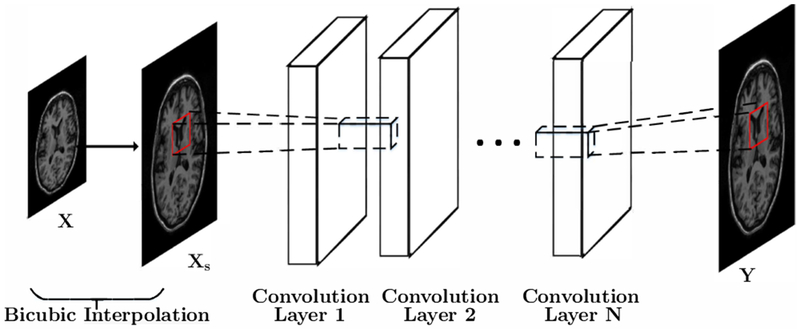
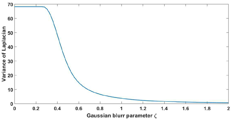
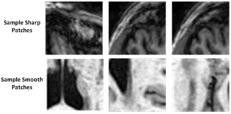
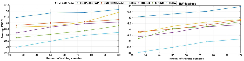
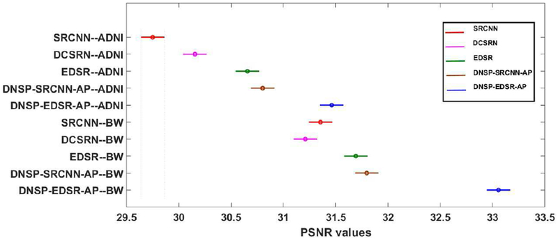
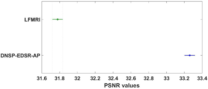
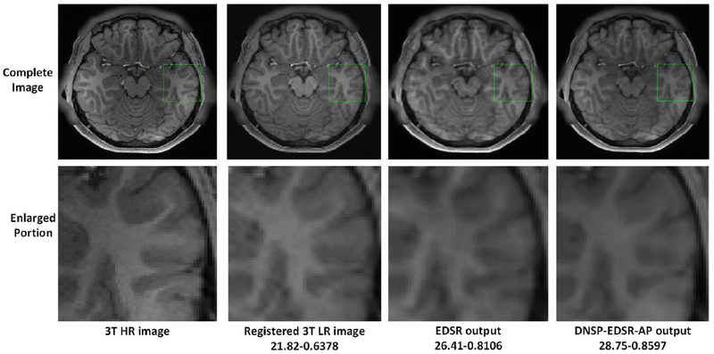
High resolution Magnetic Resonance (MR) images are desired for accurate diagnostics. In practice, image resolution is restricted by factors like hardware and processing constraints. Recently, deep learning methods have been shown to produce compelling state-of-the-art results for image enhancement/super-resolution. Paying particular attention to desired hi-resolution MR image structure, we propose a new regularized network that exploits image priors, namely a low-rank structure and a sharpness prior to enhance deep MR image super-resolution (SR). Our contributions are then incorporating these priors in an analytically tractable fashion as well as towards a novel prior guided network architecture that accomplishes the super-resolution task. This is particularly challenging for the low rank prior since the rank is not a differentiable function of the image matrix (and hence the network parameters), an issue we address by pursuing differentiable approximations of the rank. Sharpness is emphasized by the variance of the Laplacian which we show can be implemented by a fixed feedback layer at the output of the network. As a key extension, we modify the fixed feedback (Laplacian) layer by learning a new set of training data driven filters that are optimized for enhanced sharpness. Experiments performed on publicly available MR brain image databases and comparisons against existing state-of-the-art methods show that the proposed prior guided network offers significant practical gains in terms of improved SNR/image quality measures. Because our priors are on output images, the proposed method is versatile and can be combined with a wide variety of existing network architectures to further enhance their performance.

Fig. 1:

Super-Resolution CNN (SRCNN).

Fig. 2:

An example that demonstrates that MR brain images are naturally rank deficient. The low rank images are obtained by zeroing out the smallest singular values (from the SVD). This example reveals that the image has an effective rank in the range 115-120.

Fig. 3:

Variance of the Laplacian vs increasing the blur parameter.

Fig. 4:

Deep Network with Structural Priors (DNSP) for MR image super-resolution. Note the prior processing (shown in orange) is used only in the learning of the network. For a given test LR input image X, the learned SR network is used to generate the output HR image Y.

Fig. 5:

Representative examples of sharp and smooth patches. Top row represents sharp patches and bottom row represents smooth patches

Fig. 6:

The proposed DNSP architecture with learnable, data-adaptive sharpness. Bottom part of the network may be a typical state of the art LR to HR mapping, i.e. the SR network. As in Fig. 4, the parameters of the SR network are guided by prior information, except that in this case the sharpness filters are jointly learned with the network parameters Θ. Post learning, i.e. during inference, the SR network carries out the LR to HR mapping.

Fig. 7:

Illustration of EDSR architecture

Fig. 8:

Response of the 8 learned sharpness filters (along with the corresponding filter coefficients) vs. the Laplacian filter on a sample image from the ADNI dataset, as well as the coefficients of the learned filters.

Fig. 9:

Validation curves for different variations of our DNSP method on a)ADNI, and b)BW datasets. SRCNN and EDSR results are also included.

Fig. 10:

2-way ANOVA comparing DNSP vs. competing methods. The intervals represent the 95 % confidence intervals of PSNR values for a given configuration of method-dataset. Values reported for ANOVA across the method factor are d f = 7, F = 1466.94, p ⪡ .01.

Fig. 11:

Comparisons of top 4 methods for an image in BW data set for scale factor of 2. A small portion of the images (marked by green box) in the first row is zoomed in and shown in second row. The numerical figures constitute the respective PSNR-SSIM values.

Fig. 12:

Comparisons of top 4 methods for an image in ADNI dataset for scale factor of 2. A small portion of the images (marked by green box) in the first row is zoomed in and shown in second row. The numerical figures constitute the respective PSNR-SSIM values.

Fig. 13:

Comparisons of top 4 methods for an image in ADNI dataset for scale factor of 4. A small portion of the images (marked by green box) in the first row is zoomed in and shown in second row. The numerical figures constitute the respective PSNR-SSIM values.

Fig. 14:

Comparisons of top 4 methods for an image in BW data set for scale factor of 4. A small portion of the images (marked by green rectangle) in the first row is zoomed in and shown in second row. The numerical figures constitute the respective PSNR-SSIM values.

Fig. 15:

PSNR vs percent training samples.

Fig. 16:

2-way ANOVA comparing the deep learning methods for 25 percent training scenario. The intervals represent the 95 % confidence intervals of PSNR values for a given configuration of method-dataset. Values reported for ANOVA across the method factor are d f = 4, F = 362.23. p ⪡ .01.

Fig. 17:

Comparisons of LFMRI and DNSP on low field MR images. The values shown constitute the respective PSNR-SSIM values.

Fig. 18:

1-way ANOVA comparing DNSP-AP vs. EDSR for low field simulated images. The intervals represent the 95 % confidence intervals of PSNR values for a given configuration of method-dataset. Values reported for ANOVA are d f = 1, F = 439.35, p ⪡ .01.

Fig. 19:

Comparisons of EDSR and DNSP-EDSR-AP on 3T7T-DW dataset [48]. The numerical assessment is shown as PSNR-SSIM. The DNSP-EDSR generates the best results both numerically and visually compared to EDSR for 3T7T-DW dataset.

Fig. 20:

Comparisons of EDSR and DNSP-EDSR-AP on 3T3T-T1 [48]. The numerical assessment is shown as PSNR-SSIM. The DNSP-EDSR generates the best results both numerically and visually compared to EDSR for 3T3T-T1 dataset.

Fig. 21:

2-way ANOVA comparing DNSP-EDSR-AP vs. EDSR-TVLR. The intervals represent the 95 % confidence intervals of PSNR values for a given configuration of method;dataset. Values reported for ANOVA across method factor are d f = 1, F = 143.37, p ⪡ .01.

References

1. Lehmann TM, Gonner C, and Spitzer K, “Survey: Interpolation methods in medical image processing,” IEEE Trans. on Medical Imaging, vol. 18, no. 11, pp. 1049–1075, 1999. - PubMed
1. Tsai R, “Multiframe image restoration and registration,” Adv. Comput. Vis. Image Process, vol. 1, no. 2, pp. 317–339, 1984.
1. Farsiu S, Robinson MD, Elad M, and Milanfar P, “Fast and robust multiframe super resolution,” IEEE Trans. on Image Processing, vol. 13, no. 10, pp. 1327–1344, 2004. - PubMed
1. Trinh D-H, Luong M, Dibos F, Rocchisani J-M, Pham C-D, and Nguyen TQ, “Novel example-based method for super-resolution and denoising of medical images,” IEEE Trans. on Image Processing, vol. 23, pp. 1882–1895, 2014. - PubMed
1. Freeman WT, Jones TR, and Pasztor EC, “Example-based super-resolution,” Computer Graphics and Applications, vol. 22, no. 2, pp. 56–65, 2002.