Evaluation of linear and non-linear activation dynamics models for insect muscle

Abstract

In computational modelling of sensory-motor control, the dynamics of muscle contraction is an important determinant of movement timing and joint stiffness. This is particularly so in animals with many slow muscles, as is the case in insects-many of which are important models for sensory-motor control. A muscle model is generally used to transform motoneuronal input into muscle force. Although standard models exist for vertebrate muscle innervated by many motoneurons, there is no agreement on a parametric model for single motoneuron stimulation of invertebrate muscle. Although several different models have been proposed, they have never been evaluated using a common experimental data set. We evaluate five models for isometric force production of a well-studied model system: the locust hind leg tibial extensor muscle. The response of this muscle to motoneuron spikes is best modelled as a non-linear low-pass system. Linear first-order models can approximate isometric force time courses well at high spike rates, but they cannot account for appropriate force time courses at low spike rates. A linear third-order model performs better, but only non-linear models can account for frequency-dependent change of decay time and force potentiation at intermediate stimulus frequencies. Some of the differences among published models are due to differences among experimental data sets. We developed a comprehensive toolbox for modelling muscle activation dynamics, and optimised model parameters using one data set. The "Hatze-Zakotnik model" that emphasizes an accurate single-twitch time course and uses frequency-dependent modulation of the twitch for force potentiation performs best for the slow motoneuron. Frequency-dependent modulation of a single twitch works less well for the fast motoneuron. The non-linear "Wilson" model that optimises parameters to all data set parts simultaneously performs better here. Our open-access toolbox provides powerful tools for researchers to fit appropriate models to a range of insect muscles.

Fig 1. Twitch shape parameters of the Hatze-Zakotnik model.

Black to grey curves show changes in single-twitch shape with variation of parameters θ₃ (A) and θ₄ (B) in Eq 2. Parameter θ₃ modulates the twitch peak force and decay rate at a constant area under the twitch, whereas θ₄ jointly modulates peak force and single-twitch duration. Zakotnik’s extension to Hatze’s original model includes a spike-frequency-dependent modulation of parameter θ₄ (see Eq 5).

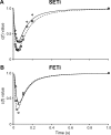
Fig 2. Modelling a single twitch.

Top row shows an isometric twitch response to a single SETi spike (blue) and corresponding model simulation results for that single twitch (solid black) using the Hatze-Zakotnik model (A) and non-linear Wilson model (B). Force is normalised to the maximum SETi-induced force of the extensor tibiae muscle of this particular animal. The spike onset is at time t = 0. The grey lines in A and C show the force responses predicted by Zajac’s first-order model, where the rise time is much shorter than in a real twitch. C, D show an isometric twitch response to a single FETi spike (red) and corresponding simulation results (black) for the same two models. Force is normalised to the maximum FETi-induced force of the extensor tibiae muscle of this particular animal. Note that for this figure, model parameters were optimised to fit the single twitch response only. In the Hatze-Zakotnik model, there were four parameters only (parameters K1 and K2 were kept constant). In the Wilson non-linear model, there were six.

Fig 3. Frequency-dependent modulation of single twitch shape can explain non-linear force potentiation.

Measured isometric force traces in response to SETi (blue, A) and FETi stimulation (red, B) and corresponding simulation using Hatze-Zakotnik model (black). Stimulation frequencies (Hz) are indicated to the right. Parameters θ₁ - θ₄ were optimised for the single twitch (as in Fig 2A and 2C) and then θ₄ was optimized separately for each spike frequency. Each SETi time course could be fitted extremely well except for the first three twitches at 10 and 12.5 Hz. For FETi, the model slightly overestimates the rise time at high frequencies and underestimates the rise time at low frequencies.

Fig 4. Frequency-dependent scaling of single twitch force.

Values of function c(t) of Eq 6 for different SETi stimulation frequencies. Black circles and solid vertical lines indicate medians and inter-quartile ranges. Smaller values indicate a stronger potentiation of twitches, with a minimum at 20 Hz (dashed line). The smaller this value, the stronger is force potentiation (see Fig 1). As a reference, the values are superimposed on a single twitch (black curve and shaded area indicate mean and inter-quartile range of experimental data, n = 5). Maximum potentiation was achieved when a spike occurred approximately 15 ms before peak twitch force generated by the preceding spike (displacement of dashed and dotted lines). The lower scale relates frequency to inter-spike interval because in Eq 5 factor c is a function of frequency, whereas in Eq 6 it is a function of time.

Fig 5. Values of force potentiation factor c as a function of inter-spike interval.

Both SETi (A) and FETi (B) panels show data from two animals (different symbols for different animals). For each symbol, factor c was calculated after frequency-specific optimisation of θ₄ to measured force traces, as shown in Fig 3. Fits are Michaelis-Menten-type functions according to Eq 6 (solid and dashed lines). Each function fit was weighted by the stimulus frequency, improving fit quality at small inter-spike intervals.

Fig 6. Constant frequency responses of five muscle activation models “as published”.

A, B show the time course of isometric SETi contractions at different stimulation frequencies (1–50 Hz) for two kinds of second-order, non-linear models: the Hatze-Zakotnik model [65] and the non-linear Wilson model ([4]. Note that, for immediate comparison, model output was normalised to maximum force of the single-twitch. This was set to 0.1. C-E show corresponding time courses of three published linear models: (C) [13], (D) [2] (both first order), and (E) [3] (third order). Constant frequency stimulation started at t = 0 s and persisted for 2 s. For comparison with FETi contractions see S4 Fig.

Fig 7. Response to random activation.

Comparison of simulated isometric SETi contraction forces in response to two Poisson spike trains with mean frequencies of 20 Hz (A) and 5 Hz (B). The same models and model parameters are used as in Fig 6. Differences between models are most prominent where force potentiation is strongest, i.e., when inter-spike intervals are approximately 50 ms. The time courses predicted by the Hatze-Zakotnik and linear Wilson models are relatively similar, as are those of the two first-order models. The non-linear Wilson model deviates most strongly from the others. For comparison with FETi contractions see S5 Fig.

Fig 8. Frequency dependence of peak isometric force.

As a summary of Fig 6 (A: SETi) and S4 Fig (B: FETi), normalised peak isometric force was plotted as a function of spike frequency for constant stimulation. Data were normalised to the peak force for a stimulation frequency of 50 Hz. For linear models, peak force linearly depends on stimulation frequency. With the published parameter sets, the Hatze-Zakotnik model has a saturating, supra-linear non-linearity for SETi stimulation, whereas the non-linear Wilson model has a sub-linear non-linearity. For FETi stimulation, both models are supra-linear, with stronger saturation for the Hatze-Zakotnik model.

Fig 9. Half-maximal rise and decay times.

Rise time to 50% of peak force at a given constant stimulation frequency for SETi (A) and FETi (B) is shown in the top row. C, D: Decay time from peak to 50% of peak force for SETi and FETi, respectively. The results were derived for the same models as used in Figs 6–8. Linear models show no frequency-dependence of decay time, and only the third-order Wilson linear model has frequency-dependent rise time. The two non-linear models differ most strongly with regard to their decay time, particularly for FETi stimulation.

Fig 10. Comparison of non-linear models optimised to the same experimental data.

Model fits (black) to experimental data sets for SETi (A, B, blue) and FETi (C, D, red) stimulation. Both models have six free parameters. Since the non-linear Wilson model optimises the complete parameter set for all force traces simultaneously, its single-twitch fit is worse than that of the Hatze-Zakotnik model. In the latter, four parameters are optimised for the single twitch, and the remaining two describe the frequency-dependent modulation of the single-twitch time course. Constant stimulation frequencies used were: 1, 7, 10, 12.5, 15, 20, 25, 30, 40 and 50 Hz for SETi, and 1, 10, 20, 30 and 50 Hz for FETi.

Fig 11. Frequency-dependent force potentiation.

Both non-linear models were fit to data from six preparations, three for SETi (A) and three for FETi (B). The experimental data range (N = 3) is shown in grey. Values were normalised to peak force obtained for stimulation at 50 Hz.

Fig 12. Half-maximal rise and decay times.

A, B: Rise time to 50% peak force at a given constant stimulation frequency for SETi (A) and FETi (B). C, D: Decay time from peak to 50% peak force for SETi (C) and FETi (D). Both models were fit to the same experimental data sets as used for Fig 11. The experimental data range is shown in grey (N = 3). No experimental data are available for frequency dependence of FETi decay. Continuous and dashed colour lines depict best-fit results for the Hatze-Zakotnik and non-linear Wilson models, respectively.

References

1. Zakotnik J, Matheson T, Dürr V (2006) Co-contraction and passive forces facilitate load compensation of aimed limb movements. J Neurosci 26: 4995–5007. 10.1523/JNEUROSCI.0161-06.2006 - DOI - PMC - PubMed
1. Blümel M, Guschlbauer C, Hooper SL, Büschges A (2012) Using individual-muscle specific instead of across-muscle mean data halves muscle simulation error. Biol Cybern 106: 573–585. 10.1007/s00422-011-0460-8 - DOI - PubMed
1. Wilson E, Rustighi E, Newland PL, Mace BR (2012) A comparison of models of the isometric force of locust skeletal muscle in response to pulse train inputs. Biomech Model Mechanobiol 11: 519–532. 10.1007/s10237-011-0330-2 - DOI - PubMed
1. Wilson E, Rustighi E, Newland PL, Mace BR (2013) Slow motor neuron stimulation of locust skeletal muscle: model and measurement. Biomech Model Mechanobiol 12: 581–596. 10.1007/s10237-012-0427-2 - DOI - PubMed
1. Clare AJ, Blackburn LML, Harischandra N, Zakotnik J, Dürr V, Matheson T (2019) Activation dynamics data for locust hind leg extensor muscle. Bielefeld University, 10.4119/unibi/2937068 - DOI
Publication types