Jensen's force and the statistical mechanics of cortical asynchronous states

Abstract

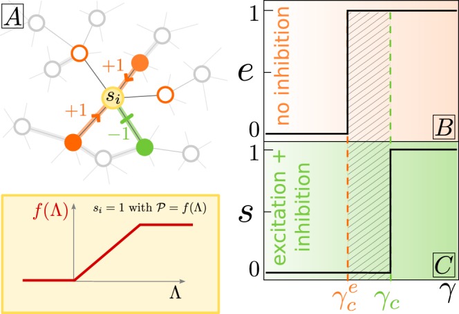
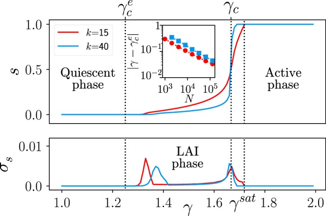
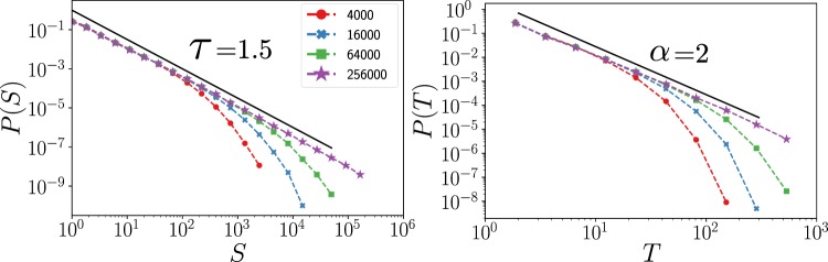
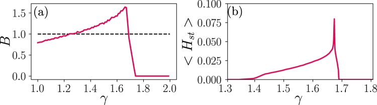
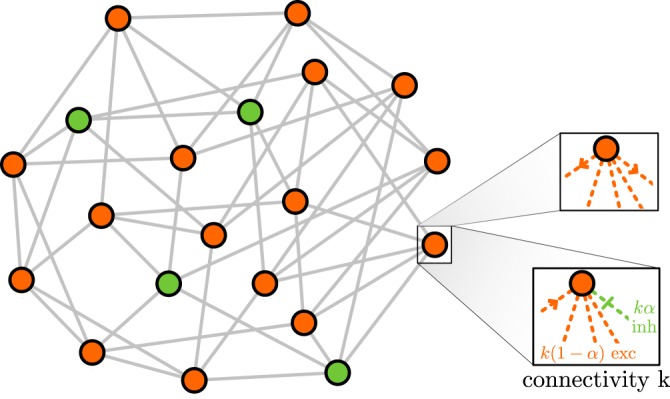
Cortical networks are shaped by the combined action of excitatory and inhibitory interactions. Among other important functions, inhibition solves the problem of the all-or-none type of response that comes about in purely excitatory networks, allowing the network to operate in regimes of moderate or low activity, between quiescent and saturated regimes. Here, we elucidate a noise-induced effect that we call "Jensen's force" -stemming from the combined effect of excitation/inhibition balance and network sparsity- which is responsible for generating a phase of self-sustained low activity in excitation-inhibition networks. The uncovered phase reproduces the main empirically-observed features of cortical networks in the so-called asynchronous state, characterized by low, un-correlated and highly-irregular activity. The parsimonious model analyzed here allows us to resolve a number of long-standing issues, such as proving that activity can be self-sustained even in the complete absence of external stimuli or driving. The simplicity of our approach allows for a deep understanding of asynchronous states and of the phase transitions to other standard phases it exhibits, opening the door to reconcile, asynchronous-state and critical-state hypotheses, putting them within a unified framework. We argue that Jensen's forces are measurable experimentally and might be relevant in contexts beyond neuroscience.

Figure 1

(A) Upper panel: Sketch of the input received by a single node, including excitatory (orange arrows) and inhibitory (green blunt arrows) interactions from active (colored) neighbors. The lower panel shows the considered transfer function for probabilistic activation of nodes as a function of the input. (B) Averaged level of activity in a fully-connected network consisting solely of $N(1-\alpha )$ excitatory nodes; it exhibits a discontinuous phase transition at ${\gamma }_c^e(\alpha )=1/(1-\alpha )$ separating a quiescent or Down state from an active or Up one. (C) As (B) but for a network consisting of $N(1-\alpha )$ excitatory and Nα inhibitory nodes. Let us remark that the shape of the phase transition depends on our choice for the transfer function. More plausible, non-linear, transfer functions lead e.g. to discontinuous transitions with a region of bistability (phase coexistence) and hysteresis; however, the main results of this work are remain unaffected (see Supplementary Information (SI) 3).

Figure 2

Overall steady-state averaged network activity s for the E/I model on a sparse hyper-regular network ($N=16,000$) in which all nodes have the same (in-)connectivity k (with either $k=15$ or $k=40$) and the same fraction of ($(1-\alpha )k$) excitatory and (αk) inhibitory inputs ($\alpha =0.2$ here). (A, Bottom) Variance across (10³) runs of the total network activity averaged in time windows of a given length ($T={10}^4$ MonteCarlo steps) as a function of the coupling strength γ for two different values of the connectivity k; each curve shows two marked peaks, indicative of two phase transitions. The leftmost one, ${\gamma }_c^e(k,N)$, shifts towards ${\gamma }_c^e$ in the large-N limit, obeying finite-size scaling, as illustrated by the straight line in the double-logarithmic plot of the inset. On the other hand, the second peak is a remanent of the mean-field first-order transition at ${\gamma }_c=1/(1-2\alpha )=1.66\dots$ and is less sensitive to finite-connectivity effects (it is always located at the point where $s=1/2$).

Figure 3

Phase diagram as a function of the coupling-strength (γ) and the connectivity k for a finite size $N=16000$ nodes. The color code indicates the level of averaged overall activity s; this shifts from the quiescent phase (reddish colors) to the active phase (blueish colors). Horizontal dashed lines correspond to the critical points ${\gamma }_c^e$ and ${\gamma }_c$ in the large-N (thermodynamic) limit. The saturation value ${\gamma }^{sat}(k)$ corresponds to Eq. (6); results from simulations are marked as black points. The curve ${\gamma }_c^e(k,N)$ represents an interpolation of the values obtained from simulations and coincides within numerical precision with the dashed line in the large-N limit.

Figure 4

Sketch illustrating the origin of the noise-induced Jensen’s force. Each node in a sparse network receives an input $\mathrm{\Lambda }$ which is a random variable extracted from some bell-shaped probability distribution function $P(\mathrm{\Lambda })$ (sketched below the x-axis) with averaged value $\langle \mathrm{\Lambda }\rangle =\gamma (1-2\alpha )s$ and standard deviation ${\sigma }_s=(\gamma \sqrt{s(1-s)})/\sqrt{k}$ (see SI-1). The possible outputs $f(\mathrm{\Lambda })$ are also distributed according to some probability (sketched to the left of the y-axis). Given that around $\mathrm{\Lambda }\approx 0$ the function $f(\mathrm{\Lambda })$ is locally convex then, as a consequence of Jensen’s inequality for convex functions, $\langle f(\mathrm{\Lambda })\rangle \ge f(\langle \mathrm{\Lambda }\rangle )$ (i.e. the dotted red line is above the blue one). Indeed, while for positive inputs, the transformation is linear, negative ones are mapped into 0 thus creating a net positive Jensen’s force for small values of $\mathrm{\Lambda }$ (or s). The inset shows the Jensen’s force $F(\tilde{\gamma },s)\equiv \langle f(\mathrm{\Lambda })\rangle >-f(\langle \mathrm{\Lambda }\rangle )$ computed right at the critical point γ_c for different connectivity values, as a function of s. Note, the negative values for large values of s which stem from the concavity of the function f(x) around x = 1. Note that F decreases as k grows and vanishes in the mean-field limit.

Figure 5

Distribution of avalanche sizes (left) and durations (right) at the (leftmost) critical point ${\gamma }_c^e$ for different system sizes (see legend) in a hyper-regular network with $k=15$. Black dotted lines are guides to the eye showing the theoretical values for an unbiased branching process.

Figure 6

(A) Time series of the excitatory (e; orange line) and inhibitory (i; green line) network activity in the LAI phase (network $N=16000$). The zoom illustrates the small (one-time step) E-I lag present in this phase. (B) Coefficient of variation (CV) vs. coupling-strength γ; $CV\ge 1$ within the LAI phase, while it vanishes in the quiescent and active phases (the color code, as in Fig. 2, stands for connectivity values). (C) Time-lagged cross-correlation (CC) between the excitation and inhibition timeseries in the LAI phase. The maximum (black dashed line) reflects the existence of a one-step E-I lag. (D) Pairwise Pearson’s correlation (PC) between nodes in the LAI phase as function of γ; it takes small values, but exhibits a marked peak at the critical point γ_c (dotted line). The inset shows that the PCs scale with system size as 1/N thus vanishing in the large-network limit (data for $\gamma =1.55$, but results valid all across the LAI phase). In all cases, we considered enough simulation runs so that errorbars are smaller than the employed symbols. Cross-Correlation and E-I lag have been obtained from a raster of $N=16000$ neurons for $t={10}^4$. The pairwise correlation is computed taking 500 random pairs, averaging over 1000 different networks.

Figure 7

(a) Branching function B in damage spreading experiments (averaged over 10⁴ runs). Black dotted lines represent marginal propagation of activity, i.e. critical dynamics. All across the LAI phase, the dynamics propagates in a chaotic way, B > 1, while in the quiescent and active phases, the Hamming distance is smaller than 1. (b) Average over runs for the time-averaged Hamming distance in the steady state $\langle H_{st}\rangle$, over $T={10}^4$ MonteCarlo steps; two initial replicas are different in a small number (10) of nodes. In this case, all across the LAI phase the difference between the two replicas $\langle H_{st}\rangle$ is very close to the steady state density, indicating that activity becomes uncorrelated between them (node states coincide only by chance). Simulations run for hyper-regular networks with $N=16,000$, $k=40$ and $\alpha =0.2$.

Figure 8

Sketch of a hyper-regular network with $N=20$ nodes and connectivity $k=5$. Orange nodes stand for excitation and green nodes for inhibition. For the zoomed node, the difference between out-activity and in-activity is also shown (i.e. each node has $k=5$ excitatory (or inhibitory) outbound links as well as $k(1-\alpha )$ excitatory and kα inhibitory inbound links). In particular, in this example, each node has 5 inbound inputs of which 4 are excitatory and 1 inhibitory, as well as 5 outbound links: all of them positive for excitatory units and negative for inhibitory ones.

References

1. Pastor-Satorras R, Castellano C, Van Mieghem P, Vespignani A. Epidemic processes in complex networks. Rev. Mod. Phys. 2015;87:925. doi: 10.1103/RevModPhys.87.925. - DOI
1. Wilson HR, Cowan JD. Excitatory and inhibitory interactions in localized populations of model neurons. Biophys. J. 1972;12:1–24. doi: 10.1016/S0006-3495(72)86068-5. - DOI - PMC - PubMed
1. Davidson E, Levin M. Gene regulatory networks. Proc. Natl. Acad. of Sci. (USA) 2005;102:4935–4935. doi: 10.1073/pnas.0502024102. - DOI - PMC - PubMed
1. Ozbudak EM, Thattai M, Lim HN, Shraiman BI, Van Oudenaarden A. Multistability in the lactose utilization network of escherichia coli. Nature. 2004;427:737. doi: 10.1038/nature02298. - DOI - PubMed
1. Isaacson JS, Scanziani M. How inhibition shapes cortical activity. Neuron. 2011;72:231–243. doi: 10.1016/j.neuron.2011.09.027. - DOI - PMC - PubMed
Publication types