Hierarchical Encoding of Attended Auditory Objects in Multi-talker Speech Perception

Abstract

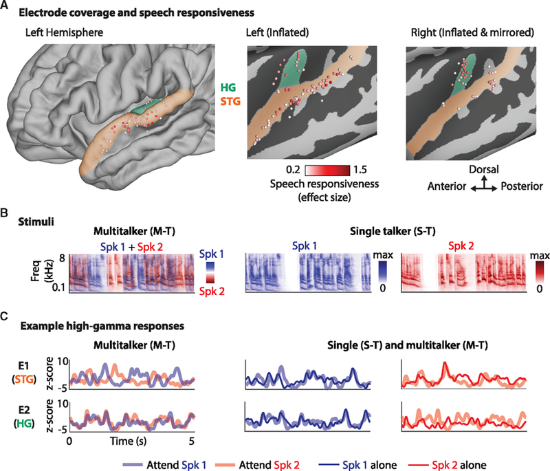
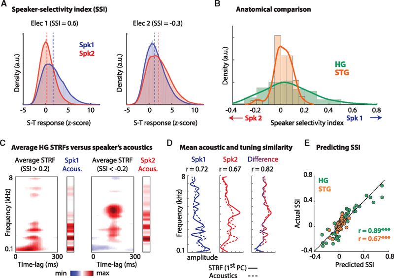
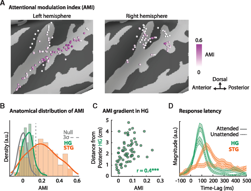
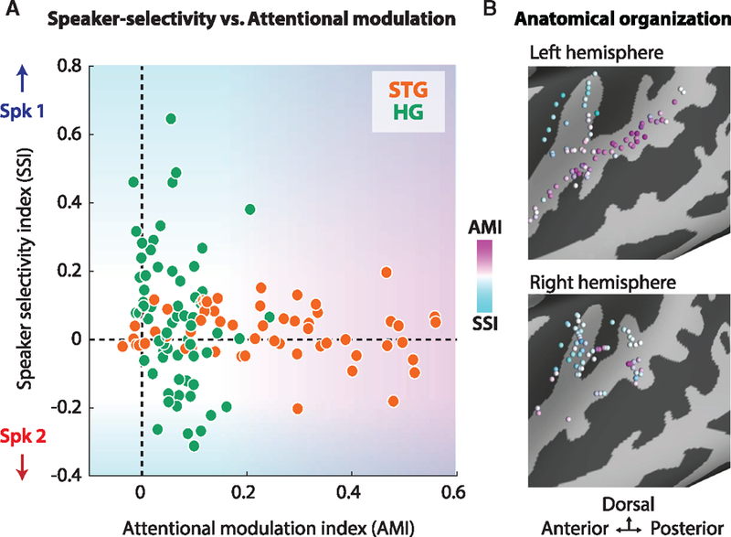
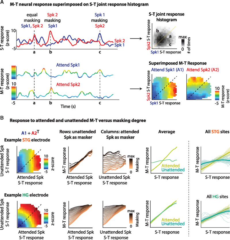
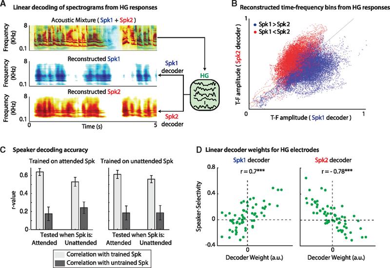
Humans can easily focus on one speaker in a multi-talker acoustic environment, but how different areas of the human auditory cortex (AC) represent the acoustic components of mixed speech is unknown. We obtained invasive recordings from the primary and nonprimary AC in neurosurgical patients as they listened to multi-talker speech. We found that neural sites in the primary AC responded to individual speakers in the mixture and were relatively unchanged by attention. In contrast, neural sites in the nonprimary AC were less discerning of individual speakers but selectively represented the attended speaker. Moreover, the encoding of the attended speaker in the nonprimary AC was invariant to the degree of acoustic overlap with the unattended speaker. Finally, this emergent representation of attended speech in the nonprimary AC was linearly predictable from the primary AC responses. Our results reveal the neural computations underlying the hierarchical formation of auditory objects in human AC during multi-talker speech perception.

Keywords: Heschl’s gyrus; auditory object; cocktail party; encoding; hierarchical; human auditory cortex; multi-talker; speech perception; superior temporal gyrus.

Figure 1.. Example of Neural Responses in Single- and Multi-talker Conditions

(A) Electrode coverage and speech responsiveness. Electrodes from all 8 subjects were transformed onto an average brain. The left panel shows the left hemisphere, with HG (containing primary auditory cortex) highlighted in green, and STG (nonprimary auditory cortex) highlighted in orange. Middle and right panels show the inflated left and right hemispheres to assist visualization. The color of each electrode corresponds to the effect size (Cohen’s D), measuring its response to speech versus silence. Only electrodes with an effect size >0.2 are shown. (B) Stimuli. Portions of the stimuli (spectrograms) in the multi-talker (left) and single-talker (middle and right) panels. In the multi-talker condition, the spectrograms of Spk1 (male) and Spk2 (female) are superimposed for visualization purposes. (C) Example neural responses from 2 electrodes in 1 subject: one in STG (e1) and the other in HG (e2). The response of e1 changes depending on which speaker is being attended, resembling the response to that speaker in isolation. Conversely, e2 responds similarly when attending to Spk1 and Spk2, as if it was responding to Spk1 alone, even when Spk2 is attended. This visualization demonstrates two response types: (1) sites with a modulated response to represent the attended speaker, and (2) sites that preferentially respond to one speaker irrespective of attention.

Figure 2.. Selective Responses of Neural Sites to Specific Speakers

(A) The distribution of the responses to Spk1 and Spk2 in the single-talker condition from 2 example electrodes in HG. Electrodes 1 and 2 respond preferentially to Spk1 and Spk2, respectively. The dashed lines indicate the median of each distribution. The speaker selectivity index (SSI) is the effect size (Cohen’s D) of the difference in the response to the 2 speakers. Positive numbers indicate a preference for Spk1, and vice versa. (B) The distribution of the SSI in HG (green) and STG (orange) shows significantly more speaker-selective sites in HG (p < 0.001). (C) Comparing the spectrotemporal tuning properties of neural sites with the acoustic profile of each speaker. Left panel: the average spectrotemporal receptive field (STRF) for all sites showing a preference for Spk1 (SSI >0.2) and the average acoustic spectrum of Spk1 (labeled Spk1 Acous.). Right panel: the average STRF for all sites showing a preference for Spk2 and the average acoustic spectrum of Spk2. (D) The correlation between the average STRFs and average acoustics (after removing the temporal component of the STRFs by obtaining their 1^st PC). Left panel: the correlation between the STRFs of Spk1 selective (SSI >0.2) sites (solid line) and the average acoustic spectrum of Spk1 (dashed line). Middle panel: the correlation between the STRFs of Spk2 selective sites and the average acoustics of Spk2. Right panel: the correlation between the difference in the 2 groups of STRFs and the difference in the acoustics of the 2 speakers. (E) Predicting the SSI of a site from its STRF for all sites in HG (green) and STG (orange).

Figure 3.. Attentional Modulation of Neural Sites

(A) The anatomical distribution of the AMI. (B) The distribution of AMI in HG (green) and STG (orange) compared with a null distribution of the AMI (gray line). A significant AMI was defined as 3 times the standard deviation of the null distribution (3σ). Significantly more sites in STG (60%) than in HG (0.06%) are modulated by attention. (C) The AMI of each site in HG compared with its distance from posterior HG. The positive correlation (r = 0.4, p < 0.001) demonstrates a gradient of attentional modulation emanating from this area. (D) The response latency of the responses in HG (green) and STG (orange; mean ± SE) with respect to the attended (solid) and unattended (dashed) speakers. These plots were obtained by averaging the STRFs across frequency to obtain the temporal response profile for each site. This result demon-strates that STG sites respond later than do HG sites and shows greater suppression of the unattended speaker.

Figure 4.. Speaker-Selectivity Index versus Attention-Modulation Index (AMI)

(A) The joint distribution of the AMI (x axis) and SSI (y axis) in HG (green) and STG (orange). This distribution further illustrates that HG shows the small effect of attention and a large amount of speaker selectivity. Conversely, STG exhibits a large effect of attention and little speaker selectivity. (B) The anatomical distribution of the SSI (cyan) and AMI (magenta). These plots illustrate a fundamental difference between the nature of the representation in HG and STG where HG provides a feature-rich, relatively static representation of the speakers, whereas STG filters out the unwanted source and selectively represents the attended speaker.

Figure 5.. The Representation of Auditory Objects in HG and STG

The magnitude of the responses in the multi-talker (M-T) condition are superimposed onto the joint distribution of the responses to Spk1 and Spk2 in the single-talker (S-T) condition. (A) For an example STG electrode, the top panel shows the responses in the S-T condition to Spk1 (blue) and Spk2 (red). The bottom panel shows the responses in the M-T condition when Spk1 is attended (top) or when Spk2 is attended (bottom). The color in these cases represents the magnitude of the response. Three time points are denoted (a, b, and c). The top-right panel shows the 2D histogram of the joint distribution of the responses to Spk1 (x axis) and Spk2 (y axis) in the S-T condition. The 3 time points (a, b, and c) and marked. In the bottom-right panel, the response magnitude of the M-T condition is superimposed on the S-T histogram (from above). The color corresponds to the response magnitude in the M-T condition. This calculation is performed separately for each attention condition (A1: attend Spk1, and A2: attend Spk2), illustrating a large effect of attention as the representation rotates 90 degrees. (B) Summarizing the responses by adding A1 to the transpose of A2. The rows of this matrix show the response to the attended speaker as the magnitude of the unattended speaker varies (changing colors), and the columns show the response to the unattended speaker as the magnitude of the attended speaker varies. This finding reveals that this site responds as a linear function of the attended speaker and is almost unaffected by the magnitude of the unattended speaker. Taking the average across the rows and columns allows for a summary of this response type (right panel). The bottom panels show the same analysis for an example electrode in HG. This finding reveals that this neural site appears to be unaffected by attention, responding linearly with respect to both speakers. The right-most panels show the average summary plots across the population of neural sites in HG and STG. This analysis reveals that (1) STG sites respond to the acoustic features of the attended speaker and are unaffected by how much these features overlap by the unattended speaker, providing evidence for the grouping of features of the attended speaker. (2) HG sites respond to the features of both speakers with no evidence of a coherent response to attended speaker features.

Figure 6.. Speakers Are Linearly Separable in HG

(A) Training linear decoders to extract either speaker from the representation of the mixture in HG. Top panel: the spectrogram of the mixture (displayed as the superposition of Spk1 and Spk2). Linear decoders can reconstruct either Spk1 (middle) or Spk2 (bottom) from the neural responses in HG to the mixture. (B) Scatterplot of the amplitude of all time-frequency (TF) bins when reconstructing Spk1 (x axis) versus reconstructing Spk2 (y axis). The dots are colored according to the dominant speaker in the corresponding T-F bin. (C) Irrespective of the actual attended speaker, both speakers can be extracted from the representation of the mixture in HG. Left panel: decoders were trained on the attended speaker and tested when that speaker was either attended or ignored (see x labels). Right panel: decoders were trained on the ignored (unattended) speaker and tested when that speaker was either attended or ignored (see x labels). Light gray bars indicate the correlation (mean ± STD) with the trained speaker, and dark gray bars indicate the correlation with the untrained speaker. In all cases, the reconstruction has a significantly higher correlation (p < 0.001) with the trained speaker than with the untrained speaker. (D) The SSI for each electrode in HG (green dots) is plotted against the average weight that the decoders learn to apply to them when the decoders are tasked with extracting Spk1 (left panel) or Spk2 (right panel). The decoders learn to enhance/suppress the electrodes that are selective for Spk1/Spk2 depending on the speaker to be extracted.

Figure 7.. Mapping HG to STG

(A) STG (orange) responds with a longer latency than HG (green), suggesting that STG is further downstream (cf. Figure 3D). (B) The neural responses in HG and STG can be predicted from the acoustic spectrogram (using a STRF) or from each other. Both areas can be predicted from the stimulus (left panel), with HG having significantly higher (p < 0.05) prediction accuracies. However, when mapping from HG to STG (and vice versa), HG can predict STG significantly better than STG can predict HG (p < 0.05). Error bars denote the mean SE. Data are from the singletalker condition. (C) Mapping HG to STG in the multi-talker condition. Left panel: for an example electrode in STG (orange dot), under attention, the weights from each HG electrode (green dots) change to enhance (suppress) the attended (unattended) speaker. Blue (red) lines correspond to a larger weight when Spk1 (Spk2) is attended. (D) The average weight change for each HG electrode (green dots) plotted against their corresponding SSI. The positive correlation (r = 0.85) confirms that larger weight changes are applied to the most speaker-selective sites in HG.

Figure 8.. Determining Speaker Selectivity in the Multi-talker Condition

Given only the representation of the mixture in HG, sites that are selective for either speaker can be determined by obtaining the correlation structure (temporal coherence) of the responses. (A) The correlation between all HG sites sorted according to their SSI. (B) Decomposing the correlation matrix in (A) using principal-component analysis (PCA) permits the acquisition of a single number for each site. The large correlation (r = 0.87) with the corresponding SSI for each electrode demonstrates that the SSI can be obtained from the multi-talker responses alone. (C) Similarly, the weights from HG to STG (HGRF) in the multi-talker condition can be determined from the same PCA analysis (r = 0.81; cf. Figure 6D).

References

1. Akbari H, Khalighinejad B, Herrero JL, Mehta AD, and Mesgarani N (2019). Towards reconstructing intelligible speech from the human auditory cortex. Sci. Rep 9, 874. - PMC - PubMed
1. Atiani S, Elhilali M, David SV, Fritz JB, and Shamma SA (2009). Task difficulty and performance induce diverse adaptive patterns in gain and shape of primary auditory cortical receptive fields. Neuron 61, 467–480. - PMC - PubMed
1. Atiani S, David SV, Elgueda D, Locastro M, Radtke-Schuller S, Shamma SA, and Fritz JB (2014). Emergent selectivity for task-relevant stimuli in higher-order auditory cortex. Neuron 82, 486–499. - PMC - PubMed
1. Bidelman GM, Moreno S, and Alain C (2013). Tracing the emergence of categorical speech perception in the human auditory system. Neuroimage 79, 201–212. - PubMed
1. Bizley JK, and Cohen YE (2013). The what, where and how of auditory-object perception. Nat. Rev. Neurosci 14, 693–707. - PMC - PubMed
Publication types
LinkOut - more resources