Kilohertz two-photon brain imaging in awake mice

Abstract

Two-photon microscopy is a mainstay technique for imaging in scattering media and normally provides frame-acquisition rates of ~10-30 Hz. To track high-speed phenomena, we created a two-photon microscope with 400 illumination beams that collectively sample 95,000-211,000 µm² areas at rates up to 1 kHz. Using this microscope, we visualized microcirculatory flow, fast venous constrictions and neuronal Ca²⁺ spiking with millisecond-scale timing resolution in the brains of awake mice.

Figure 1 ∣. Microscope design.

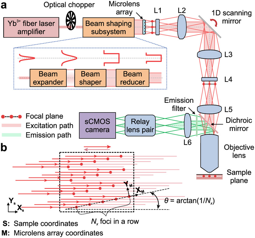
(a) A laser amplifier beam (1030 nm; ~280 fs pulse duration) passes through a chopper synchronized to the triangle-wave laser-scanning pattern (Supplementary Figs. 1,2) and is given uniform intensity across a microlens array (lenslet spacing: 100 μm), which creates N_x × N_y beamlets of equal intensity. N_x·N_y is the number of lines scanned in the specimen. Compound (L1 and L4) and aspherical lenses (L2, L3 and L5) establish intermediate and specimen focal planes (red dots: beamlet foci) as Fourier-conjugates to the plane of the scanning mirror. Fluorescence returns through the objective lens, reflects off a dichroic mirror, and is focused by a tube lens (L6) and a relay lens pair onto a sCMOS camera synchronized to the scanning mirror. Excitation and emission pathways for 3 example foci are shown in red and green, respectively. Inset: Bottom, The beam-shaper comprises an expander, a flattop shaper, and a reducer. Top, Beam intensity profiles at each stage. (b) To scan images at rates ≤1 kHz, the N_x × N_y beamlet array is projected onto the specimen at an angle, θ = tan⁻¹(1/N_x), between the (X_S, Y_S) camera-frame coordinate system (dashed rectangle) and the (X_M, Y_M) microlens array coordinate system. We generally used ≤20 × 20 laser foci (15 μm spacing between beams) oriented 2.9° to the scanning direction, yielding 0.75 μm between scanned lines. We cropped the illumination to match the area projected onto the camera.

Figure 2 ∣. Microcirculation and fast contractions of cerebral bridging veins.

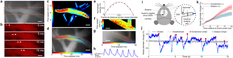
(a) Conventional epi-fluorescence image in motor cortex of an anesthetized mouse after intravenous administration of rhodamine-B. Dashed box encloses the artery in b. (b) Image time series (2.5 ms per frame; 200 kHz laser pulse rate; 2.2 mW per beamlet) taken by high-speed two-photon imaging reveals flow of injected, fluorescent HEK-293 cells. Arrowheads mark a cell’s progress. (c) Flow speed map for the vessel in b. (d) Trajectories of individual HEK-293 cells. Each trajectory is encoded in color and superposed on an epi-fluorescence image of the vasculature. (e) Flow speeds in neocortical arteries had a parabolic cross-sectional profile. For 15 different cross-sections chosen within 3 different arteries (>50 μm in diameter; N = 3 mice), we computed flow speeds, V(r), as a function of the radial deviation, r, from the vessel’s longitudinal axis. We fit (red curve) the data (blue points) to V/V_max = 1 – (r/R)ⁿ , where V_max is each vessel’s peak flow speed and R is its radius. The fitting parameter, n = 2.0 ± 0.3 (95% C.I.), revealed the flow speed’s quadratic profile. Error bars: s.e.m. (N = 15 cross-sections). (f) Flow speed map determined by 1-kHz-two-photon imaging (200 kHz laser repetition rate; 2.9 mW per beamlet; 450 × 110 μm² field of view). (g) Trajectories of individual HEK-293 cells, determined from the same dataset used for f. (h) Periodic fluctuations in blood flow, as computed within the encircled area in f. The heart rate of ~150 beats·min⁻¹ determined by high-speed imaging matches conventional measurements in ketamine-xylazine-anesthetized mice. (i) Sketch of the mouse superior sagittal sinus (SSS). Inset: We targeted areas near bregma for imaging (dotted rectangle). (j) Example time traces of bridging vein diameter determined by 200-Hz-imaging (450 × 300 μm² field of view; 200 kHz laser pulse rate; 2.2 mW per beamlet) after intravenous injection of rhodamine-B. During wakefulness, the vein diameter (blue trace) exhibited fast constriction (red dots) and dilation (cyan dots), which anesthesia abolished (gray trace). (k) Negative- and positive-going changes in vein diameter, relative to each vessel’s mean diameter, during constriction (red curve) and dilation (blue curve) in 4 awake mice. Constriction and dilation rates were, respectively, −6.5 ± 0.9% and +4.0 ± 0.7% per 100 ms (mean ± s.e.m; 36 events of each type). Shading: s.e.m. Scale bars: 50 μm in a–d, f, g.

Figure 3 ∣. High-speed Ca²⁺-imaging in neocortical and Purkinje neurons of awake mice.

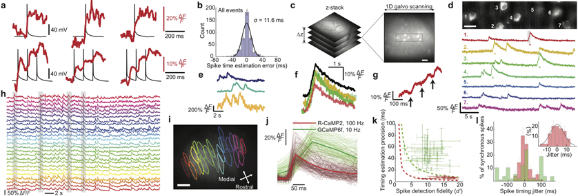
(a) To assess the spike-timing accuracy of 1-kHz-two-photon Ca²⁺-imaging, we monitored neocortical pyramidal cells in live tissue slices via whole-cell electrical recordings (black traces) and concurrent Ca²⁺-imaging (red traces; 100 kHz laser pulse rate; 0.7 mW per beamlet) using the Ca²⁺-indicator Calbryte-590. Using one or more electrical pulses (each 2 ms and 0.5–1.7 nA), we evoked individual or ≤5 successive spikes, eliciting Ca²⁺ transients. Examples of single, Top, or bursts of 3 spikes, Bottom. Stepwise increments in Ca²⁺ signals often accompanied individual spikes in a burst. (b) We estimated occurrence times of spikes and spike bursts via matched filtering of the Ca²⁺ transient waveforms, compared these to the actual times recorded electrically, and made a histogram of timing errors, aggregated across spikes and spike bursts. RMS timing error: 11.6 ms. (c) In awake mice expressing GCaMP6f in layer 2/3 cortical pyramidal cells, we first sampled a tissue volume to identify a plane suitable for 1-kHz-Ca²⁺-imaging. Boxed area (48 × 192 μm²) is magnified in d. (d) Top, We recorded the concurrent Ca²⁺ dynamics of 7 layer 2/3 neurons in an awake mouse (1-kHz-imaging; 50 kHz laser pulse rate; ~0.36 mW per beamlet). We bandpass-filtered the image with a difference of Gaussians (cutoffs: 0.42 μm and 12 μm). Scale bar: 20 μm. Bottom, Activity traces of individual cells, shown down-sampled to 500 Hz and median-filtered (time-constant: 16 ms). Asterisks mark individual Ca²⁺ transients shown in color-corresponding traces in f, g. (e) Ca²⁺ activity traces of layer 2/3 neurons in an awake mouse, acquired by 100-Hz-Ca²⁺-imaging 296 μm beneath the cortical surface (100 kHz pulse rate; 2.15 mW per beamlet). Traces were median-filtered (time constant: 200 ms). (f) Individual (colored traces) and mean (black trace) waveforms of 4 Ca²⁺ transients with asterisks in d, aligned within 4.2 ± 2.4 ms (mean ± s.d; N = 4 transients) to the onset of excitation. (g) Gray-shaded portion of the marked Ca²⁺ transient in cell 1 in d reveals a staircase-like waveform in the transient’s rising phase, similar to those seen in vitro, a, suggesting the Ca²⁺ transient accompanied a burst of spikes. (h, i) We used 100-Hz-Ca²⁺-imaging (200 kHz laser pulse rate; 2.9 mW per beamlet) to observe dendritic Ca²⁺-spiking activity of cerebellar Purkinje neurons expressing R-CaMP2 in awake mice. Example ΔF/F traces, h, of 25 neurons whose contours are shown in i superposed on a mean (0.5-min-average) two-photon image. Gray shading in h marks 4 example events when ≥80% of the visible neurons spiked synchronously. Scale bar in i: 50 μm. Field of view: 450 × 300 μm². (j) Waveforms of 492 individual Ca²⁺ spikes, after alignment of baseline fluorescence levels and spike occurrence times. Red traces: 177 randomly chosen spikes from 23 neurons imaged as in h. Green traces: 315 randomly chosen spikes from 43 Purkinje neurons imaged using GCaMP6f and conventional two-photon microscopy (10-Hz-imaging; 920 nm illumination; 30 mW). (k). By fitting a parameterized waveform to each trace in j, we found that the mean s.d. rise time to half-maximum amplitude was 13 ± 5 ms for 177 R-CaMP2 spikes imaged at 100 Hz and 50 ± 15 ms for 315 GCaMP6f spikes imaged at 10 Hz. To quantify the spike-timing estimation accuracy, we used the 95% C.I. for the model parameter setting the spike occurrence time, yielding timing accuracies of 6.8 ± 3.4 ms (mean ± s.d; 177 R-CaMP2 spikes; 100-Hz-imaging) and 48 ± 30 ms (315 GCaMP6f spikes; 10-Hz-imaging). For each Purkinje neuron, we also determined d’, the spike detection fidelity. We plotted for each cell the spike-timing accuracy versus d’ (red data points for cells studied by 100-Hz-imaging; green points for cells studied by conventional two-photon imaging). Dashed curves denote theoretical limits on spike-timing accuracy for 100-Hz-imaging (red curve) and 10-Hz-imaging on the conventional two-photon microscope (green curve), based on the Chapman-Robbins lower bound on the variance of an unbiased estimator and by approximating the 95% C.I. as twice the s.d. To calculate these limits, we used a 150 ms decay time-constant for both Ca²⁺-indicators and values from j of 30% ΔF/F for R-CaMP2 and 50% ΔF/F for GCaMP6f. Horizontal error bars: s.e.m. of each cell’s d’ value across all its spikes. Vertical error bars: s.e.m. of the 95% C.I. values across all spike occurrence times for each cell. High-speed Ca²⁺-imaging allows higher d’ values and timing accuracies within several milliseconds of the physical limitations. (l) Histogram of empirically determined timing jitters for individual spikes in synchronous spiking events, defined as instances when ≥80% of the visible Purkinje neurons spiked concurrently. We visually identified candidate events and used the methods of j to estimate spike occurrence times. We determined each spike’s jitter as the difference between its occurrence time and the mean time for all spikes in the synchronous event. The mean absolute jitter using 100-Hz-imaging and R-CaMP2 was 7.8 ± 5.5 ms (mean ± s.d.; N = 77 spikes), versus 61 ± 53 ms (N = 116 spikes) with conventional (10 Hz) two-photon imaging and GCaMP6f. Inset: Expanded view of the histogram for synchronous spikes recorded by high-speed imaging. Error bars: s.d. estimated as counting errors.