Unfold: an integrated toolbox for overlap correction, non-linear modeling, and regression-based EEG analysis

Abstract

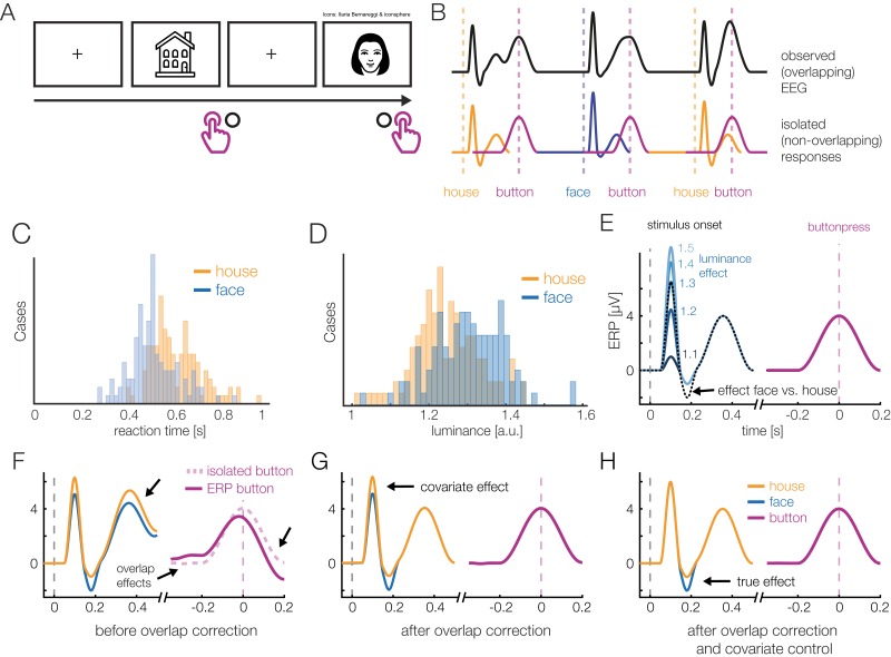
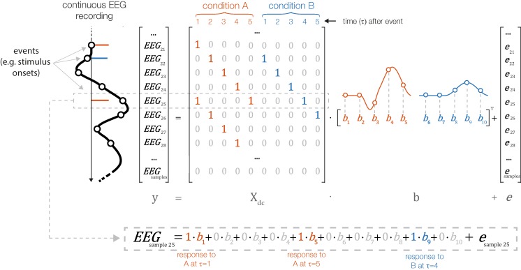
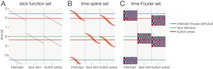
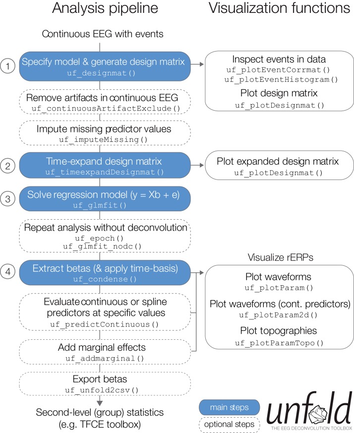
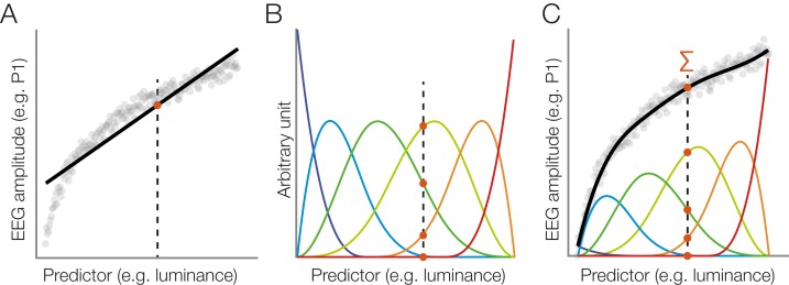
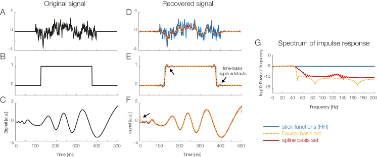
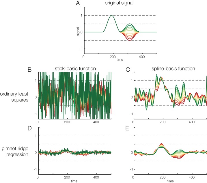
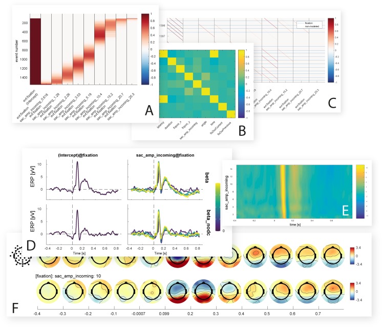
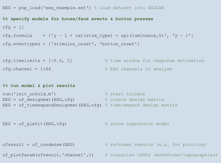
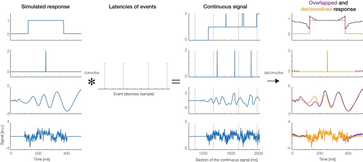
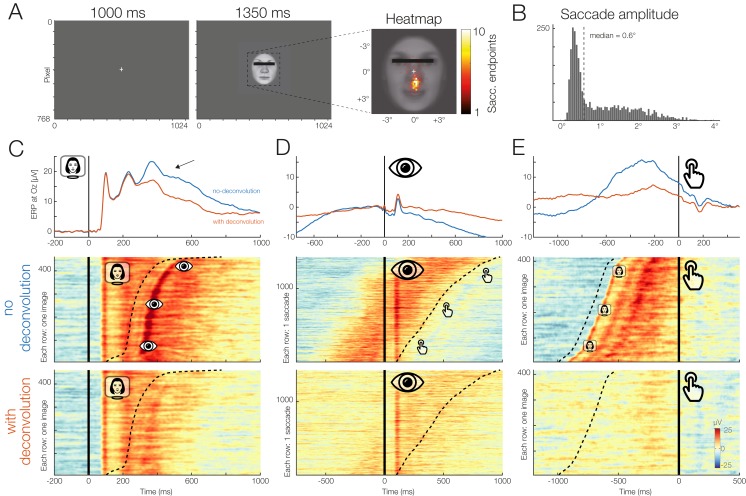
Electrophysiological research with event-related brain potentials (ERPs) is increasingly moving from simple, strictly orthogonal stimulation paradigms towards more complex, quasi-experimental designs and naturalistic situations that involve fast, multisensory stimulation and complex motor behavior. As a result, electrophysiological responses from subsequent events often overlap with each other. In addition, the recorded neural activity is typically modulated by numerous covariates, which influence the measured responses in a linear or non-linear fashion. Examples of paradigms where systematic temporal overlap variations and low-level confounds between conditions cannot be avoided include combined electroencephalogram (EEG)/eye-tracking experiments during natural vision, fast multisensory stimulation experiments, and mobile brain/body imaging studies. However, even "traditional," highly controlled ERP datasets often contain a hidden mix of overlapping activity (e.g., from stimulus onsets, involuntary microsaccades, or button presses) and it is helpful or even necessary to disentangle these components for a correct interpretation of the results. In this paper, we introduce unfold, a powerful, yet easy-to-use MATLAB toolbox for regression-based EEG analyses that combines existing concepts of massive univariate modeling ("regression-ERPs"), linear deconvolution modeling, and non-linear modeling with the generalized additive model into one coherent and flexible analysis framework. The toolbox is modular, compatible with EEGLAB and can handle even large datasets efficiently. It also includes advanced options for regularization and the use of temporal basis functions (e.g., Fourier sets). We illustrate the advantages of this approach for simulated data as well as data from a standard face recognition experiment. In addition to traditional and non-conventional EEG/ERP designs, unfold can also be applied to other overlapping physiological signals, such as pupillary or electrodermal responses. It is available as open-source software at http://www.unfoldtoolbox.org.

Keywords: EEG; ERP; Generalized additive model; Linear modeling of EEG; Non-linear modeling; Open source toolbox; Overlap correction; Regression splines; Regression-ERP; Regularization.

Figure 1. A hypothetical simple ERP experiment with overlapping responses and a non-linear covariate.

(A) A hypothetical simple ERP experiment with overlapping responses and a non-linear covariate. Data in this figure was simulated and then modeled with unfold. Participants saw pictures of faces or house and categorized them with a button press. (B) A short interval of the recorded EEG. Every stimulus onset and every button press elicits a brain response (isolated responses). However, because brain responses to the stimulus overlap with that to the response, we can only observe the sum of the overlapping responses in the EEG (upper row). (C) Because humans are experts for faces, we assume here that they reacted faster to faces than houses, meaning that the overlap with the preceding stimulus-onset ERP is larger in the face than house condition. (D) Furthermore, we assume that faces and house stimuli were not perfectly matched in terms of all other stimulus properties (e.g., spectrum, size, shape). For this example, let us simply assume that they differed in mean luminance. (E) The N170 component of the ERP is typically larger for faces than houses. In addition, however, the higher luminance alone increases the amplitude of the visual P1 component of the ERP. Because luminance is slightly higher for faces and houses, this will result in a spurious condition difference. (F) Average ERP for faces and houses, without deconvolution modeling. In addition to the genuine N170 effect (larger N170 for faces), we can see various spurious differences, caused by overlapping responses and the luminance difference. (G) Linear deconvolution corrects for the effects of overlapping potentials. (H) To also remove the confounding luminance effect, we need to also include this predictor in the model. Now we are able to only recover the true N170 effect without confounds (a similar figure was used in Dimigen & Ehinger, 2019).

Figure 2. Linear deconvolution by time expansion.

Linear deconvolution explains the continuous (toy) EEG signal within a single regression model. Specifically, we want to estimate the response (betas) evoked by each event so that together, they best explain the observed EEG. For this purpose, we create a time-expanded version of the design matrix (X_dc) in which a number of time points around each event (here: only 5 points) are added as predictors. We then solve the model for b, the betas. For instance, in the model above, sample number 25 of the continuous EEG recording can be explained by the sum of responses to three different experimental events: the response to a first event of type “A” (at time point 5 after that event), by the response to an event of type “B” (at time 4 after that event) and by a second occurrence of an event of type “A” (at time 1 after that event). Because the sequences of events and their temporal distances vary throughout the experiment, it is possible to find a unique solution for the betas that best explains the measured EEG signal. These betas, or “regression-ERPs” can then be plotted and analyzed like conventional ERP waveforms. Figure adapted from Dimigen & Ehinger (2019, with permission).

Figure 3. Temporal basis functions.

Overview over different temporal basis functions. The expanded design matrix X_dc is plotted, the y-axis represents time and the x-axis shows all time-expanded predictors in the model. In unfold, three methods are available for time expansion: (A) Stick-functions. Here, each modeled time point relative to the event is represented by a unique predictor. (B) Time-splines allow neighboring time points to smooth themselves. This generally results in less predictors than the stick function set. (C) Truncated time-Fourier set: It is also possible to use a Fourier basis. By omitting high frequencies from the Fourier-set, the data are effectively low-pass filtered during the deconvolution process (see also Fig. 6).

Figure 4. Overview over typical analysis steps with unfold.

The first step is to load a continuous EEG dataset into EEGLAB. This dataset should already contain event markers (e.g., for stimulus onsets, button presses, etc.). Afterwards there are four main analysis steps, that can be executed with a few lines of code (see also Box 1). These steps, highlighted in blue, are: (1) Define the model formula and let unfold generate the design matrix, (2) time-expand this design matrix, (3) solve the model to obtain the betas (i.e., rERPs), and (4) convert the betas into a convenient format for plotting and statistics. The right column lists several inbuilt plotting functions to visualize intermediate analysis steps or to plot the results (see also Fig. 8).

Figure 5. Modeling a non-linear relationship with a set of spline functions.

(A) Example of a non-linear relationship between a predictor (e.g., stimulus luminance) and a dependent variable (e.g., EEG amplitude). A linear function (black line) does not fit the data well. We will follow one luminance value (dashed line) at which the linear function is evaluated (red dot). (B) Instead of a linear fit, we define a set of overlapping spline functions which are distributed across the range of the predictor. In this example, we are using a set of six b-splines. For our luminance value, we receive six new predictor values. Only three of them are non-zero. (C) We weight each spline with its respective estimated beta value. To predict the dependent variable (EEG amplitude) at our luminance value (dashed line), we sum up the weighted spline functions (red dots). Because the splines are overlapping, this produces a smooth, non-linear fit to the observed data.

Figure 6. Using temporal basis functions.

Effect of using different time basis functions on the recovery of the original signal using deconvolution. (A–C) Show three different example signals without deconvolution (in black) and with convolution using different methods for the time-expansion (stick, Fourier, spline). We zero-padded the original signal to be able to show boundary artifacts. For the analysis we used 45 time-splines and in order to keep the number of parameters equivalent, the first 22 cosine and sine functions of the Fourier set. The smoothing effects of using a time-basis set can be best seen in the difference between the blue curve and the orange/red curves in (D). Artifacts introduced due to the time-basis set are highlighted with arrows and can be seen best in (E) and (F). Note that in the case of realistic EEG data, the signal is typically smooth, meaning that ripples like in (E) rarely occur. (G) The impulse response spectrum of the different smoothers. Clearly, the Fourier-set filters better than the splines, but splines allow for a sparser description of the data and could benefit in the fitting stage.

Figure 7. Regularization options.

Effects of regularization on deconvolving noisy data. Results of regularization are shown both for a model with stick-functions and for a model with a temporal spline basis set. (A) To create an overlapped EEG signal, we convolved 38 instances of the original signal depicted in (A). The effect of a continuous covariate was randomly added to each event (see different colors in A). To make the data noisy, we added Gaussian white noise with a standard deviation of 1. Finally, to illustrate the power of regularization, we also added another random covariate to the model. This covariate had no relation to the EEG signal but was highly correlated (r = 0.85) to the first covariate. Thus, the model formula was: EEG ∼ 1 + covariate + randomCovariate. (B) Parameters recovered based on ordinary least squares regression. Due to the low signal-to-noise ratio of the data, the estimates are extremely noisy. (C) Some smoothing effect can be achieved by using time-splines as a temporal basis set instead of stick functions. (D) The same data, but deconvolved using a L2-regularized estimate (ridge regression). It is obvious that the variance of the estimate is a lot smaller. However, compared to the original signal shown in (A), the estimated signal is also much weaker, i.e., there is a strong bias. (E) L2-regularized estimates, computed with a time-spline basis set. This panel shows the usefulness of regularization: the effect structure can be recovered despite strong noise, although the recovered effect is again strongly biased (due to the variance/bias tradeoff).

Figure 8. Inbuilt data visualization options.

Shown are some of the figures currently produced by the unfold toolbox. While setting up the model, it is possible to visualize intermediate steps of the analysis, such as the design matrix (A) covariance matrix of the predictors (B) or the time-expanded design matrix (C). After the model is computed, the beta coefficients for one or more predictors can be plotted as ERP-like waveforms with a comparison of with and without deconvolution (D), as ERP images with time against predictor value and color-coded amplitude (E), or as topographical time series (F).

Figure 9. A complete analysis script with unfold.

For further documentation and interactive tutorials visit https://www.unfoldtoolbox.org.

Figure 10. Deconvolution results for simulated signals.

Four types of responses (first column: box car, Dirac function, auditory ERP, pink noise) were convolved with random event latencies (second column). A section of the resulting overlapped signal is shown in the third column. The fourth column shows the deconvolved response recovered by the unfold toolbox (orange lines). Overlapped responses (without deconvolution) are plotted as violet lines for comparison.

Figure 11. Example dataset with stimulus onsets, eye movements, and button presses.

(A) Panel adapted from Dimigen & Ehinger (2019). The participant was shown a stimulus for 1,350 ms. (B) The subject was instructed to keep fixation, but as the heatmap shows, made many small involuntary saccades towards the mouth region of the presented stimuli. Each saccade also elicits a visually-evoked response (lambda waves). (C–E) Latency-sorted and color-coded single-trial potentials at electrode Oz over visual cortex (second row) reveal that the vast majority of trials contain not only the neural response to the face (C) but also hidden visual potentials evoked by involuntary microsaccades (D) as well as motor potentials from preparing the button press (E). Deconvolution modeling with unfold allows us to isolate and remove these different signal contributions (see “no deconvolution” vs. “with deconvolution”), resulting in corrected ERP waveforms for each process (blue vs. red waveforms). This reveals, for example, that a significant part of the P300 evoked by faces (arrow in (C)) is really due to microsaccades and button presses and not the stimulus presentation.

References

1. Alday PM. How much baseline correction do we need in ERP research? Extended GLM model can replace baseline correction while lifting its limits. Psychophysiology. 2019;94(1):206. doi: 10.1111/psyp.13451. - DOI - PubMed
1. Amsel BD. Tracking real-time neural activation of conceptual knowledge using single-trial event-related potentials. Neuropsychologia. 2011;49(5):970–983. doi: 10.1016/j.neuropsychologia.2011.01.003. - DOI - PubMed
1. Baayen HR, Davidson DJ, Bates DM. Mixed-effects modeling with crossed random effects for subjects and items. Journal of Memory and Language. 2007;59(4):390–412. doi: 10.1016/j.jml.2007.12.005. - DOI
1. Bach DR, Flandin G, Friston KJ, Dolan RJ. Time-series analysis for rapid event-related skin conductance responses. Journal of Neuroscience Methods. 2009;184(2):224–234. doi: 10.1016/j.jneumeth.2009.08.005. - DOI - PMC - PubMed
1. Bigdely-Shamlo N, Touyran J, Ojeda A, Kothe C, Mullen T, Robbins K. Automated EEG mega-analysis II: cognitive aspects of event related features. BiorXiv. 2018 doi: 10.1101/411371. - DOI - PubMed