A chromosome folding intermediate at the condensin-to-cohesin transition during telophase

Abstract

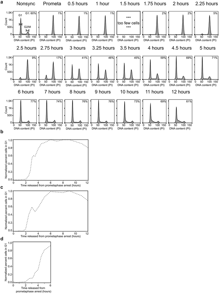
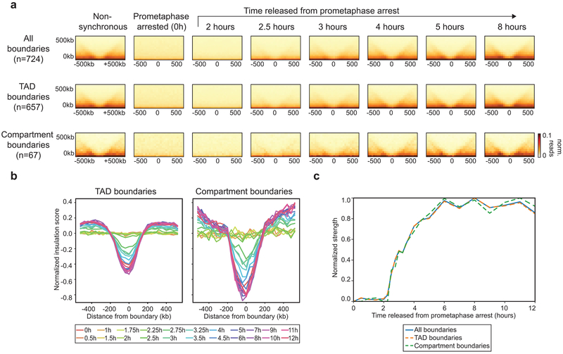
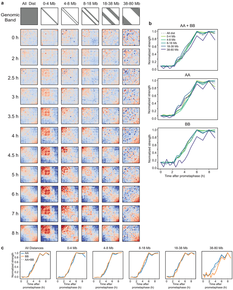
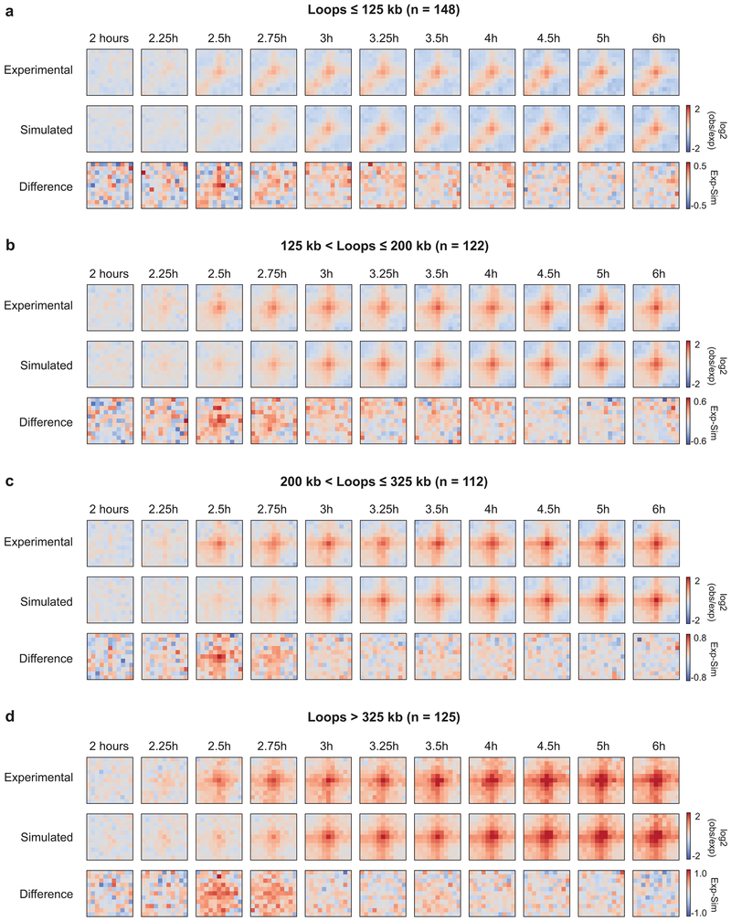
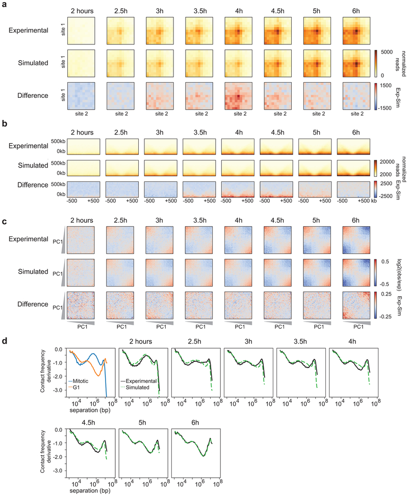
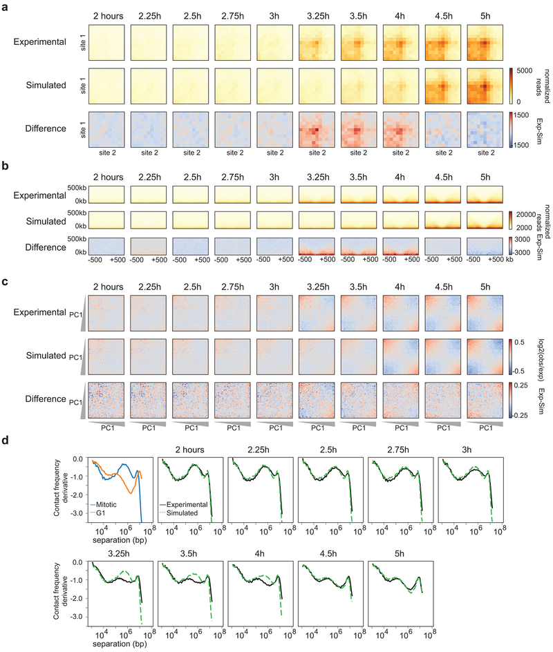
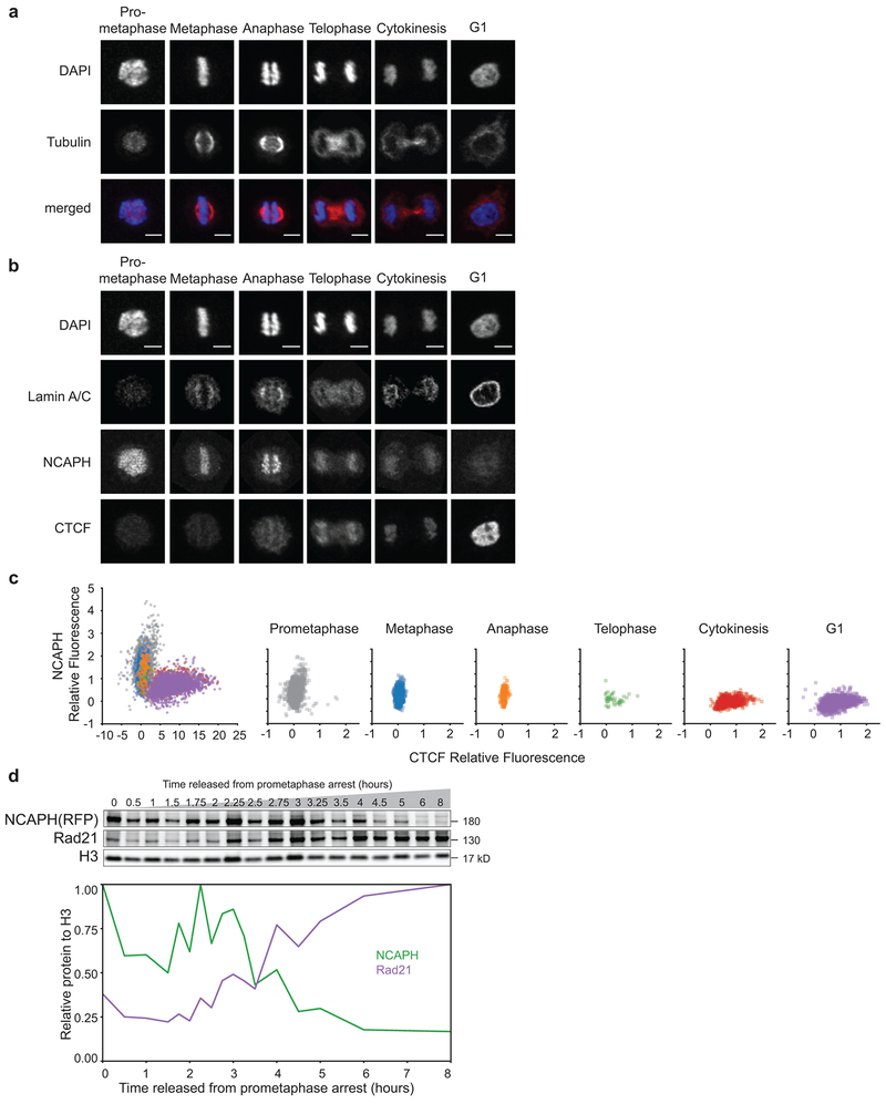
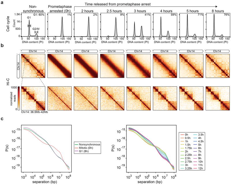
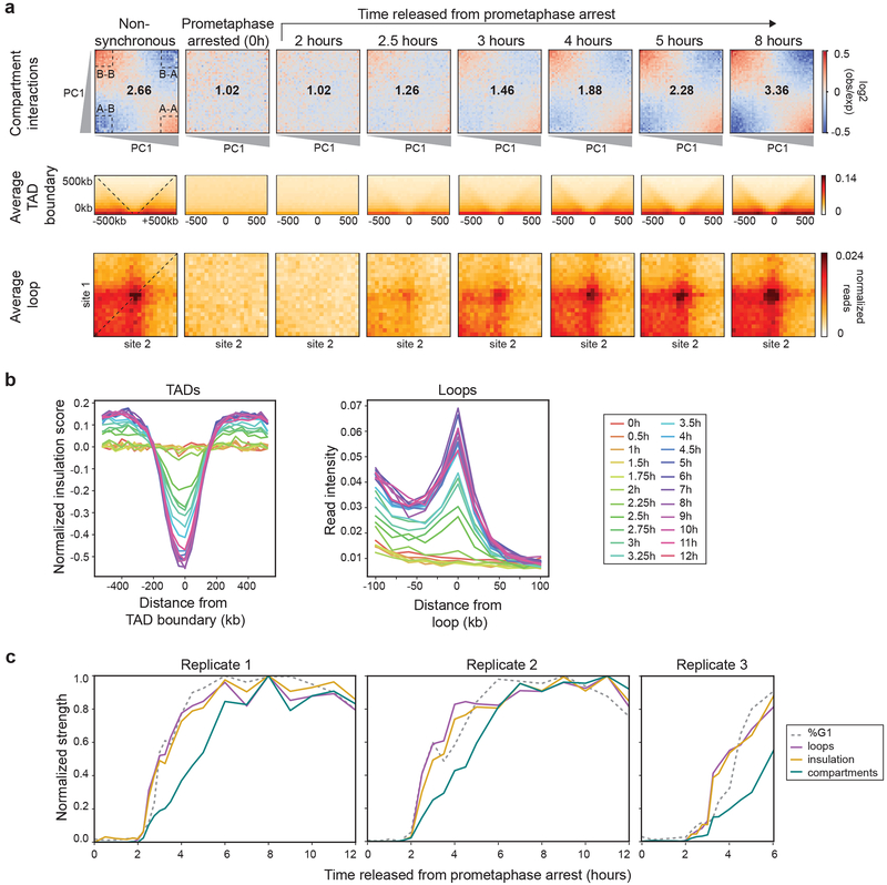
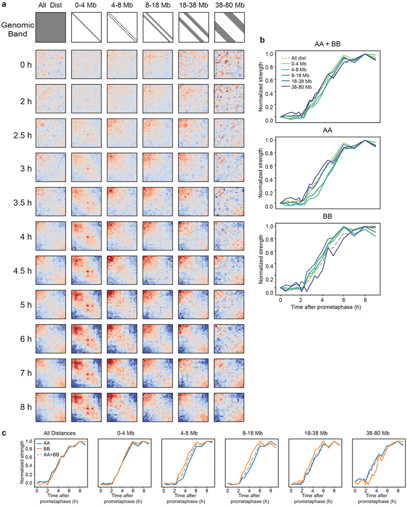
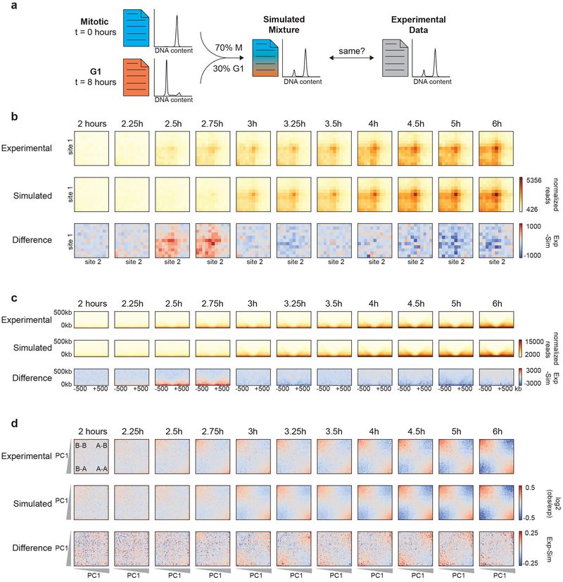
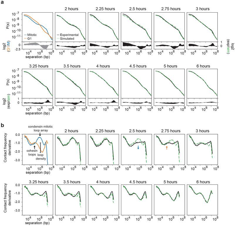
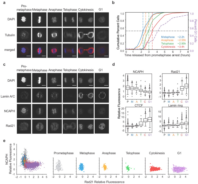
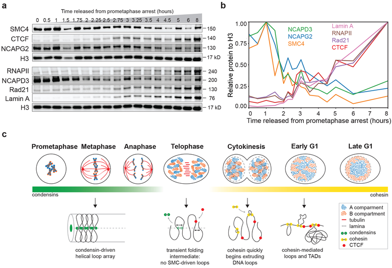
Chromosome folding is modulated as cells progress through the cell cycle. During mitosis, condensins fold chromosomes into helical loop arrays. In interphase, the cohesin complex generates loops and topologically associating domains (TADs), while a separate process of compartmentalization drives segregation of active and inactive chromatin. We used synchronized cell cultures to determine how the mitotic chromosome conformation transforms into the interphase state. Using high-throughput chromosome conformation capture (Hi-C) analysis, chromatin binding assays and immunofluorescence, we show that, by telophase, condensin-mediated loops are lost and a transient folding intermediate is formed that is devoid of most loops. By cytokinesis, cohesin-mediated CTCF-CTCF loops and the positions of TADs emerge. Compartment boundaries are also established early, but long-range compartmentalization is a slow process and proceeds for hours after cells enter G1. Our results reveal the kinetics and order of events by which the interphase chromosome state is formed and identify telophase as a critical transition between condensin- and cohesin-driven chromosome folding.

Extended Data Fig. 1. Cell cycle analysis of mitotic exit time courses

a, FACS analysis of nonsynchronous and prometaphase-arrested cultures and of cultures at different time points after release from prometaphase-arrest in time course replicate 1. Percentages in the upper right corner represent the number of cells with a G1 DNA content. b-d, Quantification of the fraction of cells in G1 at each time point from time course replicate 1 normalized to t = 8 hours (b), time course replicate 2 normalized to t = 8 hours (c), and time course replicate 3 normalized to a G1 maximum assumed to be 80% (d). Three independent experiments were performed with similar results. Source Data are provided in Source data Extended Data Fig. 1.

Extended Data Fig. 2. Compartment analysis for time course replicate 1

a, Principal component 1 (PC1) along Chromosome 14 for Hi-C data obtained from cells at different time points after release from prometaphase. Principal component analysis was performed on Hi-C data binned at 200 kb resolution. PC1 detects A and B compartments starting at t = 3 hours. Lower left corner represents Pearson correlation value of each track compared to nonsynchronous PC1. b, Principal component 3 (PC3) along Chromosome 14 for Hi-C data obtained from cells at different time points after release from prometaphase. Principal component analysis was performed on Hi-C data binned at 200 kb resolution. PC3 detects some A and B compartments starting at t = 2.75 hours, but at later time points, PC1 captures compartments. Lower left corner represents Pearson correlation value of each track compared to nonsynchronous PC1. Three independent experiments were performed with similar results.

Extended Data Fig. 3. TAD and compartment domain boundaries form with similar kinetics

a, Aggregate Hi-C data binned at 40 kb resolution at domain boundaries (top = all 724 boundaries, middle = 657 TAD boundaries, bottom = 67 compartment boundaries) at different time points after release from prometaphase. b, Average insulation profile across averaged domain boundaries shown in panel a (left = TAD boundaries, right = compartment boundaries) for different time points. c, Normalized strength for domain boundaries as a function of time after release from prometaphase. The strength for each of these features was set at 1 for the 8 hour time point. TAD boundaries and compartment boundaries form with similar kinetics. Three independent replicate experiments yielded similar results. Source Data are provided in Source Data Extended Data Fig. 3.

Extended Data Fig. 4. Compartment analysis for chromosome 14

a, Saddle plots of Hi-C data for chromosome 14 binned at 200 kb resolution for different time points and split into genomic distance bands, as shown in gray in the first row. b, Normalized compartmentalization strength of different genomic distances as a function of time and split by interaction type (A-A, B-B, A-B). c, Normalized compartmentalization strength of interaction types as a function of time and split by genomic distance. Three independent experiments were performed with similar results. Source Data are provided in Source data Extended Data Fig. 4.

Extended Data Fig. 5. Kinetics of loop formation for loops of different size

Loops were grouped according to size: a, loops less than or equal to 125 kb, b, loops greater than 125 kb and less than or equal to 200 kb, c, loops greater than 200 kb and less than or equal to 325 kb, d, loops greater than 325 kb. For each panel, top row: log2(observed/expected) Hi-C data for experimental time course, middle row: log2(observed/expected) Hi-C data for simulated time course, bottom row: the difference between experimental and simulated Hi-C data. Kinetics of loop formation is similar for all loop sizes. Three independent experiments were performed with similar results.

Extended Data Fig. 6. Analysis of time course replicate 2

a, Aggregated Hi-C data binned at 20 kb resolution at chromatin loops at different time points. Top row: Experimental Hi-C data. Middle row: Simulated Hi-C data. Bottom row: The difference between experimental and simulated Hi-C data. Loops are more prominent in experimental Hi-C data than in the simulated data between 3 and 4.5 hours. This analysis included loops larger than 200 kb to avoid the strong signal at the diagonal of the interaction matrix. Simulations were performed with experimental data from this time course (mixing Hi-C data for t = 0 and t = 8 hours). b, Aggregate Hi-C data binned at 40 kb resolution at TAD boundaries for different time points. Top row: Experimental Hi-C data. Middle row: Simulated Hi-C data. Bottom row: The difference between experimental and simulated Hi-C data. Insulation strength is stronger in experimental Hi-C data than in simulated Hi-C data at t = 3.5 and t = 4.5 hours. c, Saddle plots of Hi-C data binned at 200 kb resolution for different time points. Top row: Experimental Hi-C data. Middle row: Simulated Hi-C data. Bottom row: The difference between experimental and simulated Hi-C data. Compartmentalization is weaker in experimental Hi-C than in simulated Hi-C data as illustrated by the fact that A-B interactions are less depleted in the experimental data (upper right and lower left corner of saddle plots). d, Derivative from P(s) plots. Black lines represent the derivative of P(s) for experimental Hi-C data and the dashed green lines represent the derivative of P(s) for the simulated Hi-C datasets for corresponding time points. Three independent experiments were performed with similar results.

Extended Data Fig. 7. Analysis of time course replicate 3

a, Aggregated Hi-C data binned at 20 kb resolution at chromatin loops at different time points. Top row: Experimental Hi-C data. Middle row: Simulated Hi-C data. Bottom row: The difference between experimental and simulated Hi-C data. Loops are more prominent in experimental Hi-C data than in the simulated data between 3.25 and 4 hours. This analysis included loops larger than 200 kb to avoid the strong signal at the diagonal of the interaction matrix. Simulations were performed with experimental data from this time course (mixing Hi-C data for t = 0 and t = 6 hours). b, Aggregate Hi-C data binned at 40 kb resolution at TAD boundaries for different time points. Top row: Experimental Hi-C data. Middle row: Simulated Hi-C data. Bottom row: The difference between experimental and simulated Hi-C data. Insulation strength is stronger in experimental Hi-C data than in simulated Hi-C data at t = 3.25 and t = 4 hours. c, Saddle plots of Hi-C data binned at 200 kb resolution for different time points. Top row: Experimental Hi-C data. Middle row: Simulated Hi-C data. Bottom row: The difference between experimental and simulated Hi-C data. Compartmentalization is weaker in experimental Hi-C than in simulated Hi-C data as illustrated by the fact that A-B interactions are less depleted in the experimental data (upper right and lower left corner of saddle plots). d, Derivative from P(s) plots. Black lines represent the derivative of P(s) for experimental Hi-C data and the dashed green lines represent the derivative of P(s) for the simulated Hi-C datasets for corresponding time points. Three independent experiments were performed with similar results.

Extended Data Fig. 8. Chromatin association dynamics of CTCF, condensin, and cohesion

a, Classification of cell cycle stages based on DAPI staining and tubulin organization. Scale bar = 5μm. b, Localization of Lamin A/C, NCAPH, and CTCF during different cell cycle stages shown in panel a. Scale bar = 5μm. c, Quantification of CTCF and NCAPH colocalization with chromatin in single cells at different cell cycle stages. Left plot represents data from all cells with color indicating cell cycle stage. Right plots represent the data separated into each individual cell cycle stage. d, Top: Western blot analysis of chromatin-associated proteins purified from HeLaS3-NCAPH-dTomato cells at different time points after release from prometaphase. Bottom: Quantification of the western blot shown above. NCAPH and Rad21 were analyzed on the same gel. The samples for Histone H3 analysis were run on another gel. Four independent experiments were performed with similar results. Source Data for microscopy are provided in Source data Fig. 7. Unprocessed blots are provided in Source data Extended Data Fig. 8.

Fig. 1:. Hi-C analysis during mitotic exit and G1 entry

a, FACS analysis of nonsynchronous and prometaphase-arrested cultures and of cultures at different time points after release from prometaphase-arrest. Percentages in the upper right corner represent the percent of cells with a G1 DNA content. Replicate time courses yielded similar results (Extended Data 1c-d). b, Hi-C interaction maps for nonsynchronous and prometaphase-arrested cultures and of cultures at different time points after release from prometaphase-arrest. The order of panels is the same as in a. Data for chromosome 14 are shown for two resolutions: 200 kb (top row, for entire right arm) and 40 kb (bottom row, for 36.5 Mb – 42 Mb region). Hi-C heatmaps are all on the same color scale. c, Left: P(s) plots for Hi-C data from nonsynchronous, mitotic (t = 0 hours), or G1 (t = 8 hours) cultures. Right: P(s) plots for Hi-C data from cells at indicated time points after release from prometaphase. Three independent experiments were performed with similar results.

Fig. 2:. Kinetics of loop, TAD, and compartment formation

a, Top row: Saddle plots of Hi-C data binned at 200 kb resolution for nonsynchronous and prometaphase-arrested cultures and of cultures at different time points after release from prometaphase-arrest. Saddle plots were calculated using the PC1 obtained from the Hi-C data of the 8 hour time point. Numbers at the center of the heatmaps indicate compartment strength calculated as the ratio of (AA+BB)/(AB+AB) using the mean values from dashed corner boxes. Middle row: Aggregate Hi-C data binned at 40 kb resolution at TAD boundaries identified from the Hi-C data of the 8 hour time point (n = 724 boundaries). The order of panels is the same as the top row. Dashed lines indicate the edges of the averaged domains. Bottom row: Aggregate Hi-C data binned at 10 kb resolution at chromatin loops on intact HeLa S3 chromosomes (n = 507 loops) identified in Rao et al. . The order of panels is the same as the top row. b, Left: Average insulation profile across TAD boundaries shown in panel a for different time points. Right: Average Hi-C signals at and around looping interactions. Each line represents the signal from the lower left corner to the upper right corner of the loop aggregate heatmaps shown in panel a (dashed line). c, Normalized feature strength for TADs, loops, and compartments as a function of time after release from prometaphase. For replicate time course 1 (left) and replicate time course 2 (middle) the strength of each of these features was set at 1 for the 8 hour time point. Dotted line indicates the fraction of cells in G1 at each time point, normalized to t = 8 hours. For replicate time course 3 (right) the strength for each of these features was normalized to the strength expected based on data from replicate 1. Dotted line indicates the fraction of cells in G1 at each time point, normalized to G1 maximum assumed to be 80%. Three independent experiments were performed with similar results. Source Data are provided in Source data Fig. 2.

Fig. 3:. Kinetics of A and B compartment formation at various genomic distances

a, Saddle plots of Hi-C data for the right arm of chromosome 4 binned at 200 kb resolution for different time points and split into genomic distance bands, as shown in gray in the first row. b, Normalized compartmentalization strength of different genomic distances as a function of time and split by interaction type (A-A, B-B, A-B). c, Normalized compartmentalization strength of interaction types as a function of time and split by genomic distance. Three independent experiments were performed with similar results. Source Data are provided in Source data Fig. 3.

Fig. 4:. TADs and loops form quicker than expected, while compartmentalization occurs slower than expected

a, Schematic diagram of simulating Hi-C data based on the percentage of G1 cells at each time point. b, Aggregate Hi-C data binned at 20 kb resolution at chromatin loops at different time points. Top row: Experimental Hi-C data. Middle row: Simulated Hi-C data. Bottom row: The difference between experimental and simulated Hi-C data. Loops are more prominent in experimental Hi-C data than in the simulated data at t = 2.5 and t = 2.75 hours. This analysis included loops larger than 200 kb to avoid the strong signal at the diagonal of the interaction matrix. c, Aggregate Hi-C data binned at 40 kb resolution at TAD boundaries for different time points. Top row: Experimental Hi-C data. Middle row: Simulated Hi-C data. Bottom row: The difference between experimental and simulated Hi-C data. Insulation strength is stronger in experimental Hi-C data than in simulated Hi-C data at t = 2.5 and t = 2.75 hours. d, Saddle plots of Hi-C data binned at 200 kb resolution for different time points. Top row: Experimental Hi-C data. Middle row: Simulated Hi-C data. Bottom row: The difference between experimental and simulated Hi-C data. Saddle plots were calculated using the PC1 obtained from the experimental Hi-C data of the 8 hour time point. Compartmentalization is weaker in experimental Hi-C than in simulated Hi-C data as illustrated by the fact that A-B interactions are less depleted in the experimental data (upper right and lower left corner of saddle plots). Similar results were obtained with independent experimental and corresponding simulated time courses (Extended Data 6a-c, 7a-c). Three independent experiments were performed with similar results.

Fig. 5:. Formation of a transient folding intermediate

a, Contact frequency (P) versus genomic distance (s) for read normalized Hi-C datasets for experimental mitotic and G1 data (upper left, blue and orange lines, respectively) and experimental Hi-C data obtained from cells at different time points after release from prometaphase arrest (black lines). Dashed green lines are P(s) plots for simulated Hi-C datasets for corresponding time points. At the bottom of each P(s) plot, the difference between experimental and simulated P(s) is plotted for the different time points, except for the upper left plot which shows the difference P(s) for experimental G1 and mitotic cells. Note that the difference plot for the upper left graph is on a different scale than all of the other difference plots. b, Derivative from P(s) plots shown in panel a. In the upper left graph, we indicate features that represent the condensin mitotic loop array and the cohesin loop size and density. The blue arrow indicates loss of the condensin-dependent mitotic loop array. The orange arrow indicates the initiation of the cohesin-dependent G1 loops. Similar results were obtained with independent experimental and corresponding simulated time courses (Extended Data 6d, 7d). Three independent experiments were performed with similar results.

Fig. 6:. Chromatin colocalization dynamics of condensins and cohesin during mitotic exit

a, Representative images of classification of cell cycle stages based on DAPI staining and tubulin organization (see Methods). Scale bar = 5 μm. b, Cumulative plots of HeLaS3-NCAPH-dTomato cells at different cell cycle stages (left axis) and the percent of cells in G1 (right axis) defined by imaging. At least 400 individual cells were classified for each time point: 0 minutes (n = 405 cells), 30m (n = 520), 60m (n = 780), 90m (n = 669), 105m (n = 638), 120m (n = 613), 135m (n = 601), 150m (n = 812), 165m (n = 533), 180m (n = 507), 195m (n = 650), 210m (n = 607), 240m (n = 1057), 270m (n = 760), 300m (n = 855), 360m (n = 1186), 480m (n = 959). c, Localization of Lamin A/C, NCAPH, and Rad21 during different cell cycle stages shown in panel a. Scale bar = 5 μm. For images showing CTCF localization see Extended Data 8a-b. d, Quantification of NCAPH, Rad21 and CTCF colocalization with chromatin and lamin ring formation at different cell cycle stages (see Methods). P = prometaphase, M = metaphase, A = anaphase, T = telophase, C = cytokinesis, G1 = G1. Box plots represent quartiles of the dataset with a line at the median value, whiskers represent range of the dataset, and diamonds outside of whiskers are outliers. Cell numbers for CTCF plot were P (n = 2099 cells), M (n = 1020), A (n = 199), T (n = 39), C (n = 853), and G1 (n = 2142) (see Extended Data 8a-b). For the other three plots, the corresponding numbers were 1601, 1052, 155, 74, 927, and 2100. e, Quantification of Rad21 and NCAPH colocalization with chromatin in single cells at different cell cycle stages. Left plot represents data from all cells with color indicating cell cycle stage. Right plots represent the data separated into each individual cell cycle stage. Four independent experiments were performed with similar results. Source Data are provided in Source data Fig. 6.

Fig. 7:. Chromatin association dynamics of condensins and cohesin during mitotic exit

a, Western blot analysis of chromatin-associated proteins purified from HeLa S3 cells at different time points after release from prometaphase. b, Quantification of the western blot shown in panel a. Protein levels were normalized to Histone H3 levels from the same samples. c, Summary of cellular and chromosomal events as cells exit mitosis and enter G1. Top: Schematic diagrams indicate the cellular events from prometaphase into late G1. Compartment type is indicated by color: blue = A, orange = B. Red lines represent tubulin and dashed gray lines represent lamina. Bottom: Models of chromosome conformation during early mitosis, telophase, cytokinesis, and interphase. Green bar indicates abundance of condensins I and II on the chromatin at the corresponding cell cycle stages. Yellow bar indicates cohesin abundance on the chromatin at the corresponding cell cycle stages. Unprocessed blots are provided in Source Data as Unprocessed Blots Figure 7. Four independent experiments were performed with similar results. Source Data are provided in Source data Fig. 7.

References

1. Fudenberg G, Abdennur N, Imakaev M, Goloborodko A & Mirny LA Emerging Evidence of Chromosome Folding by Loop Extrusion. Cold Spring Harb Symp Quant Biol 82, 45–55 (2017). - PMC - PubMed
1. Rao SSP et al. A 3D map of the human genome at kilobase resolution reveals principles of chromatin looping. Cell 159, 1665–1680 (2014). - PMC - PubMed
1. de Wit E et al. CTCF Binding Polarity Determines Chromatin Looping. Mol Cell. 60, 676–684 (2015). - PubMed
1. Guo Y et al. CRISPR Inversion of CTCF Sites Alters Genome Topology and Enhancer/Promoter Function. Cell 162, 900–910 (2015). - PMC - PubMed
1. Vietri Rudan M et al. Comparative Hi-C reveals that CTCF underlies evolution of chromosomal domain architecture. Cell Rep. 10, 1297–1309 (2015). - PMC - PubMed
Publication types