Global atmospheric CO2 inverse models converging on neutral tropical land exchange, but disagreeing on fossil fuel and atmospheric growth rate

Abstract

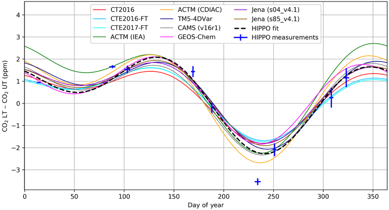
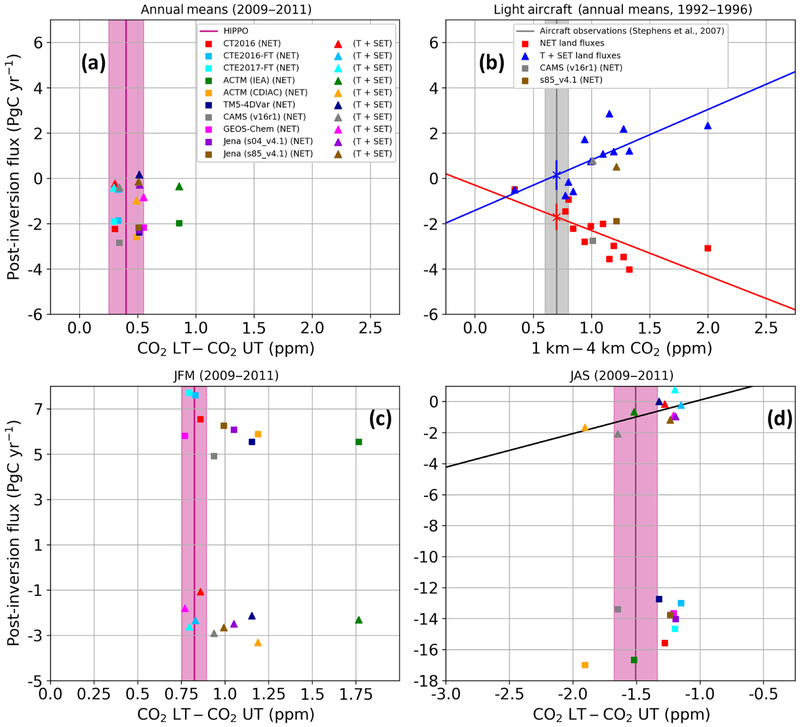
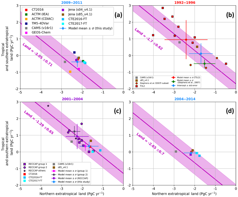
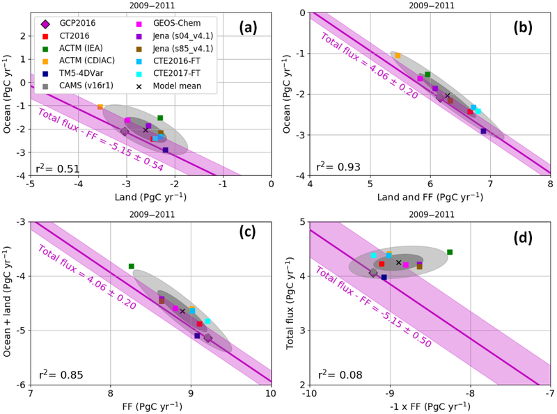
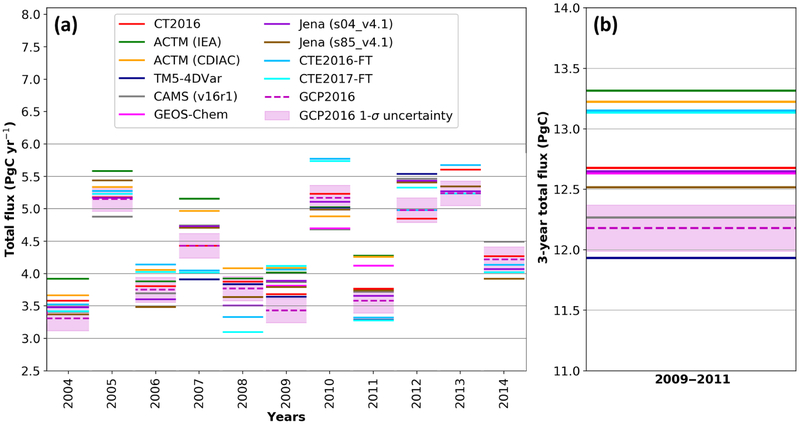
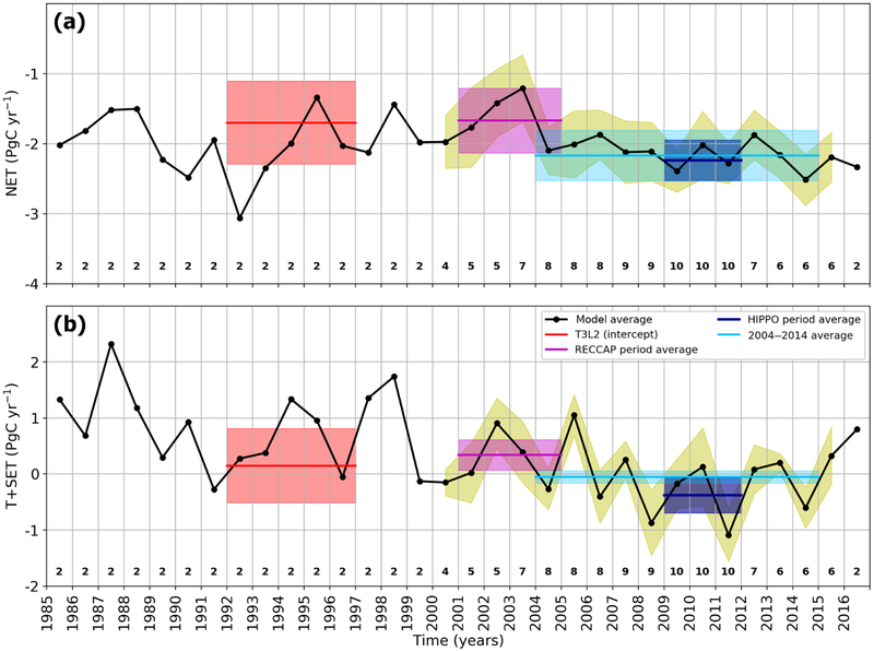
We have compared a suite of recent global CO₂ atmospheric inversion results to independent airborne observations and to each other, to assess their dependence on differences in northern extratropical (NET) vertical transport and to identify some of the drivers of model spread. We evaluate posterior CO₂ concentration profiles against observations from the High-Performance Instrumented Airborne Platform for Environmental Research (HIAPER) Pole-to-Pole Observations (HIPPO) aircraft campaigns over the mid-Pacific in 2009-2011. Although the models differ in inverse approaches, assimilated observations, prior fluxes, and transport models, their broad latitudinal separation of land fluxes has converged significantly since the Atmospheric Carbon Cycle Inversion Intercomparison (TransCom 3) and the REgional Carbon Cycle Assessment and Processes (RECCAP) projects, with model spread reduced by 80% since TransCom 3 and 70% since RECCAP. Most modeled CO₂ fields agree reasonably well with the HIPPO observations, specifically for the annual mean vertical gradients in the Northern Hemisphere. Northern Hemisphere vertical mixing no longer appears to be a dominant driver of northern versus tropical (T) annual flux differences. Our newer suite of models still gives northern extratropical land uptake that is modest relative to previous estimates (Gurney et al., 2002; Peylin et al., 2013) and near-neutral tropical land uptake for 2009-2011. Given estimates of emissions from deforestation, this implies a continued uptake in intact tropical forests that is strong relative to historical estimates (Gurney et al., 2002; Peylin et al., 2013). The results from these models for other time periods (2004-2014, 2001-2004, 1992-1996) and reevaluation of the TransCom 3 Level 2 and RECCAP results confirm that tropical land carbon fluxes including deforestation have been near neutral for several decades. However, models still have large disagreements on ocean-land partitioning. The fossil fuel (FF) and the atmospheric growth rate terms have been thought to be the best-known terms in the global carbon budget, but we show that they currently limit our ability to assess regional-scale terrestrial fluxes and ocean-land partitioning from the model ensemble.

Figure 1.

Reconstructed annual cycle in northern extratropical vertical CO₂ gradients, obtained from fits using two harmonics of the HIPPO data and correspondingly sampled model outputs, averaged over 20 to 90° N (1000 to 800 hPa minus 800 to 400 hPa). The CO₂ average curtain observations for each of nine atmospheric transects have been added on the graph to illustrate the data uncertainties and temporal coverage, the y-axis error bar is derived from the range of disagreement among the three in situ instruments on board (QCLS, OMS, and AO2; see Supplement), and the line average is derived from the CO2.X merged dataset. The horizontal whiskers represent the time span of the flights contributing to each average. The observed line shown here is not a direct fit to the observation points, but rather comes from an average of fits to individual 100 hPa by 5° latitude bins as described in the text.

Figure 2.

Retrieved fluxes versus NET vertical gradients. (a) Annual mean NET land and T+SET land fluxes versus posterior NET vertical gradients (lower minus upper troposphere) from model output along HIPPO flight tracks and HIPPO observations (pink line) for the period 2009–2011. The shaded area represents an estimate of measurement uncertainty of ±0.15 ppm for the annual mean, as estimated in the Sect. S2 in the Supplement. Inverse model posterior concentration gradients and fluxes are shown as points (squares represent NET; triangles represent T+SET). The vertical axis represents the integrated annual mean land fluxes (PgC yr⁻¹). (b) Same as (a) but for 1992–1996 and showing TransCom 3 Level 2 models and our two current models that span this time period, showing dependence of posterior fluxes on transport and a large range of transport biases. Annual mean NET (red squares) and T+SET (blue triangles) land carbon fluxes for 1992–1996 estimated by the 12 T3L2 models plotted as a function of the models’ post-inversion predicted mean vertical CO₂ gradients at 10 light-aircraft profiling sites (adapted from Stephens et al., 2007) with fluxes partitioned by TransCom region. The Jena (s85_v4.1) and the CAMS (v16r1) simulations have also been sampled at the same light-aircraft locations but their fluxes are partitioned at 20° N and 20° S. The crosses show our new best estimate of the fluxes estimated by the regression of all T3L2 models. The error bars on these points are estimated using the standard error of the regressions. (c) Same as panel (a) for January–February–March (JFM), and (d) same as panel (a) for July–August–September (JAS). For the seasonal plots, the width of the pink bar is 0.07 ppm for JFM and 0.17 for JAS. In panel (d), the black line represents the regression line, shown because the relationship is statistically significant at a 95% confidence interval.

Figure 3.

Tropical and southern extratropical (T+SET) versus northern extratropical (NET) land fluxes for the periods (a) 2009–2011, (b) 1992–1996, (c) 2001–2004, and (d)2004–2014. The new models used in this study are represented by squares and the average of the available or selected simulations is shown in blue with 1 standard deviation error bars. The pink line and shaded area represents the GCP2016 (river adjusted) estimates of the total land sink for the given period. (a) Results for the HIPPO period 2009–2011; (b) results for the T3L2 period 1992–1996. The TransCom 3 Level 2 outputs (Gurney et al., 2004) are shown in red, with the vertical gradient selected models from Stephens et al. (2007) as circles outlined in green and the rest as red squares outlined in black. The intercept of the regression line with the observed vertical gradient (Fig. 2) is used to define our best flux estimate with error bars estimated by the standard error of the linear regression. (c) Results for the RECCAP period 2001–2004. Also, from Peylin et al. (2013), model means and standard deviations are shown in pink for the subgroup 1 (Jena, LSCEa, MACC-II, CTE2013, CT2011_oi) and in gray for the subgroup 2 (MATCH, CCAM, TrC, NICAM). Panel (d) shows the results from our new set of models for the period 2004–2014.

Figure 4.

Synthesis of globally integrated fluxes for the 2009–2011 period, in PgC yr⁻¹. Each inversion is represented by a square and the model mean by a × symbol. The GCP2016 estimates are a pink diamond, which is sometimes hard to see because it is superimposed in each panel by the gray CAMS point. We have adjusted the GCP2016 ocean and land flux estimates by the riverine flux of carbon from land to ocean to atmosphere (0.45 PgC yr⁻¹; Jacobson et al., 2007; Le Quéré et al., 2018), decreasing the ocean sink and increasing the land sink. The magenta line and light-pink shaded area show the corresponding mass balance estimates from GCP2016. In each panel the line and equation shown represent the sum of the x and y variables, and thus the line has a slope of −1, and any deviation perpendicular to the line indicates disagreement on the sum. Here we use the total flux which by mass balance is the whole-atmosphere growth rate (see text), and for panels (a) and (d), the total flux – FF line also equals O + L, while for panels (b) and (c), the total flux line equals O + L + FF. Ellipses denote the variability around the model means of 1σ (darker gray) and 2σ (lighter gray). (a) Ocean versus land; (b) ocean versus land + FF; (c) ocean + land versus FF; (d) total flux versus − 1 × FF.

Figure 5.

Modeled total flux (lines), equal to whole-atmosphere growth rate, that is the difference between the global FF emissions and the land and ocean fluxes. Atmospheric growth rate from GCP2016, derived from atmospheric CO₂ measurements made in the marine boundary layer by the NOAA ESRL flask network (Masarie and Tans, 1995; Dlugokencky and Tans, 2018) and GCP2016 assigned uncertainty (pink bands). (b) Shows the sum of the total flux for the 3 years (2009 to 2011).

Figure 6.

Time series of annual land fluxes for the NET (a) and the T+SET (b). The black line represents the model mean and standard deviation derived from available simulations; the number of simulations is shown by the numbers below the curve. The standard deviation is shown only if there are more than two model simulations available. Estimates from the specific period (Table 2) are added as multi-year average and standard deviation (shaded area).

References

1. Ammoura L, Xueref-Remy I, Vogel F, Gros V, Baudic A, Bonsang B, Delmotte M, Té Y, and Chevallier F: Exploiting stagnant conditions to derive robust emission ratio estimates for CO2, CO and volatile organic compounds in Paris, Atmos. Chem. Phys, 16, 15653–15664, 10.5194/acp-16-15653-2016, 2016. - DOI
1. Ballantyne AP, Alden CB, Miller JB, Tans PP, and White JWC: Increase in observed net carbon dioxide uptake by land and oceans during the past 50 years, Nature, 488, 70–72, 10.1038/nature11299, 2012. - DOI - PubMed
1. Ballantyne AP, Andres R, Houghton R, Stocker BD, Wanninkhof R, Anderegg W, Cooper LA, DeGrandpre M, Tans PP, Miller JB, Alden C, and White JWC: Audit of the global carbon budget: estimate errors and their impact on uptake uncertainty, Biogeosciences, 12, 2565–2584, 10.5194/bg-12-2565-2015, 2015. - DOI
1. Bastos A, Running SW, Gouveia C, and Trigo RM: The global NPP dependence on ENSO: La Nina and the extraordinary year of 2011, J. Geophys. Res.-Biogeo, 118, 1247–1255, 10.1002/jgrg.20100, 2013. - DOI
1. Basu S, Guerlet S, Butz A, Houweling S, Hasekamp O, Aben I, Krummel P, Steele P, Langenfelds R, Torn M, Biraud S, Stephens B, Andrews A, and Worthy D: Global CO2 fluxes estimated from GOSAT retrievals of total column CO2, Atmos. Chem. Phys, 13, 8695–8717, 10.5194/acp-13-8695-2013, 2013. - DOI
LinkOut - more resources